below is the xample file # ================= Polynomial Regression =================== # Thus far, we have assumed that the relationship between the explanatory # variables and the response variable is linear. This assumption is not always # true. This is where polynomial regression comes in. Polynomial regression # is a special case of multiple linear regression that adds terms with degrees # greater than one to the model. The real-world curvilinear relationship is captured # when you transform the training data by adding polynomial terms, which are then fit in # the same manner as in multiple linear regression. # We are now going to us only one explanatory variable, but the model now has # three terms instead of two. The explanatory variable has been transformed # and added as a third term to the model to captre the curvilinear relationship. # The PolynomialFeatures transformer can be used to easily add polynomial features # to a feature representation. Let's fit a model to these features, and compare it # to the simple linear regression model: import numpy as np import matplotlib.pyplot as plt from sklearn.linear_model import LinearRegression from sklearn.preprocessing import PolynomialFeatures # Training set x_train = [[6], [8], [10], [14], [18]] #diamters of pizzas y_train = [[7], [9], [13], [17.5], [18]] #prices of pizzas # Testing set x_test = [[6], [8], [11], [16]] #diamters of pizzas y_test = [[8], [12], [15], [18]] #prices of pizzas # Train the Linear Regression model and plot a prediction regressor = LinearRegression() regressor.fit(x_train, y_train) xx = np.linspace(0, 26, 100) yy = regressor.predict(xx.reshape(xx.shape[0], 1)) plt.plot(xx, yy) # Set the degree of the Polynomial Regression model quadratic_featurizer = PolynomialFeatures(degree = 2) # This preprocessor transforms an input data matrix into a new data matrix of a given degree X_train_quadratic = quadratic_featurizer.fit_transform(X_train) X_test_quadratic = quadratic_featurizer.transform(x_test) # Train and test the regressor_quadratic model regressor_quadratic = LinearRegression() regressor_quadratic.fit(X_train_quadratic, y_train) xx_quadratic = quadratic_featurizer.transform(xx.reshape(xx.shape[0], 1)) # Plot the graph plt.plot(xx, regressor_quadratic.predict(xx_quadratic), c = 'r', linestyle = '--') plt.title('Pizza price regressed on diameter') plt.xlabel('Diameter in inches') plt.ylabel('Price in dollars') plt.axis([0, 25, 0, 25]) plt.grid(True) plt.scatter(X_train, y_train) plt.show() print (X_train) print (X_train_quadratic) print (X_test) print (X_test_quadratic) # If you execute the code, you will see that the simple linear regression model is plotted with # a solid line. The quadratic regression model is plotted with a dashed line and evidently # the quadratic regression model fits the training data better.
below is the xample file # ================= Polynomial Regression =================== # Thus far, we have assumed that the relationship between the explanatory # variables and the response variable is linear. This assumption is not always # true. This is where polynomial regression comes in. Polynomial regression # is a special case of multiple linear regression that adds terms with degrees # greater than one to the model. The real-world curvilinear relationship is captured # when you transform the training data by adding polynomial terms, which are then fit in # the same manner as in multiple linear regression. # We are now going to us only one explanatory variable, but the model now has # three terms instead of two. The explanatory variable has been transformed # and added as a third term to the model to captre the curvilinear relationship. # The PolynomialFeatures transformer can be used to easily add polynomial features # to a feature representation. Let's fit a model to these features, and compare it # to the simple linear regression model: import numpy as np import matplotlib.pyplot as plt from sklearn.linear_model import LinearRegression from sklearn.preprocessing import PolynomialFeatures # Training set x_train = [[6], [8], [10], [14], [18]] #diamters of pizzas y_train = [[7], [9], [13], [17.5], [18]] #prices of pizzas # Testing set x_test = [[6], [8], [11], [16]] #diamters of pizzas y_test = [[8], [12], [15], [18]] #prices of pizzas # Train the Linear Regression model and plot a prediction regressor = LinearRegression() regressor.fit(x_train, y_train) xx = np.linspace(0, 26, 100) yy = regressor.predict(xx.reshape(xx.shape[0], 1)) plt.plot(xx, yy) # Set the degree of the Polynomial Regression model quadratic_featurizer = PolynomialFeatures(degree = 2) # This preprocessor transforms an input data matrix into a new data matrix of a given degree X_train_quadratic = quadratic_featurizer.fit_transform(X_train) X_test_quadratic = quadratic_featurizer.transform(x_test) # Train and test the regressor_quadratic model regressor_quadratic = LinearRegression() regressor_quadratic.fit(X_train_quadratic, y_train) xx_quadratic = quadratic_featurizer.transform(xx.reshape(xx.shape[0], 1)) # Plot the graph plt.plot(xx, regressor_quadratic.predict(xx_quadratic), c = 'r', linestyle = '--') plt.title('Pizza price regressed on diameter') plt.xlabel('Diameter in inches') plt.ylabel('Price in dollars') plt.axis([0, 25, 0, 25]) plt.grid(True) plt.scatter(X_train, y_train) plt.show() print (X_train) print (X_train_quadratic) print (X_test) print (X_test_quadratic) # If you execute the code, you will see that the simple linear regression model is plotted with # a solid line. The quadratic regression model is plotted with a dashed line and evidently # the quadratic regression model fits the training data better.

Database System Concepts
7th Edition
ISBN:9780078022159
Author:Abraham Silberschatz Professor, Henry F. Korth, S. Sudarshan
Publisher:Abraham Silberschatz Professor, Henry F. Korth, S. Sudarshan
Chapter1: Introduction
Section: Chapter Questions
Problem 1PE

Related questions

Question
below is the xample file
# ================= Polynomial Regression ===================
# Thus far, we have assumed that the relationship between the explanatory
# variables and the response variable is linear. This assumption is not always
# true. This is where polynomial regression comes in. Polynomial regression
# is a special case of multiple linear regression that adds terms with degrees
# greater than one to the model. The real-world curvilinear relationship is captured
# when you transform the training data by adding polynomial terms, which are then fit in
# the same manner as in multiple linear regression.
# We are now going to us only one explanatory variable, but the model now has
# three terms instead of two. The explanatory variable has been transformed
# and added as a third term to the model to captre the curvilinear relationship.
# The PolynomialFeatures transformer can be used to easily add polynomial features
# to a feature representation. Let's fit a model to these features, and compare it
# to the simple linear regression model:
import numpy as np
import matplotlib.pyplot as plt
from sklearn.linear_model import LinearRegression
from sklearn.preprocessing import PolynomialFeatures
# Training set
x_train = [[6], [8], [10], [14], [18]] #diamters of pizzas
y_train = [[7], [9], [13], [17.5], [18]] #prices of pizzas
# Testing set
x_test = [[6], [8], [11], [16]] #diamters of pizzas
y_test = [[8], [12], [15], [18]] #prices of pizzas
# Train the Linear Regression model and plot a prediction
regressor = LinearRegression()
regressor.fit(x_train, y_train)
xx = np.linspace(0, 26, 100)
yy = regressor.predict(xx.reshape(xx.shape[0], 1))
plt.plot(xx, yy)
# Set the degree of the Polynomial Regression model
quadratic_featurizer = PolynomialFeatures(degree = 2)
# This preprocessor transforms an input data matrix into a new data matrix of a given degree
X_train_quadratic = quadratic_featurizer.fit_transform(X_train)
X_test_quadratic = quadratic_featurizer.transform(x_test)
# Train and test the regressor_quadratic model
regressor_quadratic = LinearRegression()
regressor_quadratic.fit(X_train_quadratic, y_train)
xx_quadratic = quadratic_featurizer.transform(xx.reshape(xx.shape[0], 1))
# Plot the graph
plt.plot(xx, regressor_quadratic.predict(xx_quadratic), c = 'r', linestyle = '--')
plt.title('Pizza price regressed on diameter')
plt.xlabel('Diameter in inches')
plt.ylabel('Price in dollars')
plt.axis([0, 25, 0, 25])
plt.grid(True)
plt.scatter(X_train, y_train)
plt.show()
print (X_train)
print (X_train_quadratic)
print (X_test)
print (X_test_quadratic)
# If you execute the code, you will see that the simple linear regression model is plotted with
# a solid line. The quadratic regression model is plotted with a dashed line and evidently
# the quadratic regression model fits the training data better.
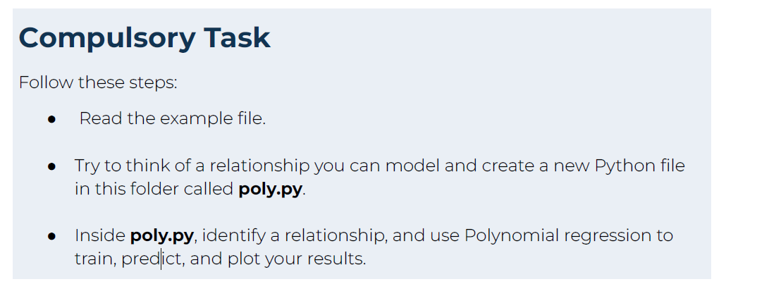
Transcribed Image Text:Compulsory Task
Follow these steps:
Read the example file.
• Try to think of a relationship you can model and create a new Python file
in this folder called poly.py.
Inside poly.py, identify a relationship, and use Polynomial regression to
train, predict, and plot your results.
Expert Solution
This question has been solved!
Explore an expertly crafted, step-by-step solution for a thorough understanding of key concepts.

Step by step
Solved in 4 steps with 2 images

Knowledge Booster


Learn more about
Need a deep-dive on the concept behind this application? Look no further. Learn more about this topic, computer-science and related others by exploring similar questions and additional content below.Recommended textbooks for you
Database System Concepts
Computer Science
ISBN:
9780078022159
Author:
Abraham Silberschatz Professor, Henry F. Korth, S. Sudarshan
Publisher:
McGraw-Hill Education

Starting Out with Python (4th Edition)
Computer Science
ISBN:
9780134444321
Author:
Tony Gaddis
Publisher:
PEARSON

Digital Fundamentals (11th Edition)
Computer Science
ISBN:
9780132737968
Author:
Thomas L. Floyd
Publisher:
PEARSON
Database System Concepts
Computer Science
ISBN:
9780078022159
Author:
Abraham Silberschatz Professor, Henry F. Korth, S. Sudarshan
Publisher:
McGraw-Hill Education
Starting Out with Python (4th Edition)
Computer Science
ISBN:
9780134444321
Author:
Tony Gaddis
Publisher:
PEARSON
Digital Fundamentals (11th Edition)
Computer Science
ISBN:
9780132737968
Author:
Thomas L. Floyd
Publisher:
PEARSON

C How to Program (8th Edition)
Computer Science
ISBN:
9780133976892
Author:
Paul J. Deitel, Harvey Deitel
Publisher:
PEARSON

Database Systems: Design, Implementation, & Manag…
Computer Science
ISBN:
9781337627900
Author:
Carlos Coronel, Steven Morris
Publisher:
Cengage Learning

Programmable Logic Controllers
Computer Science
ISBN:
9780073373843
Author:
Frank D. Petruzella
Publisher:
McGraw-Hill Education