1. Create a vector of time ranging from 0 to 41 seconds with an increment of 0.01 seconds between points. Suppress output to the command window. 2. Evaluate the function ℎ(??) at the points in the time vector using element-by-element math. Suppress output to the command window. 3. Create a new figure window and plot the height versus time of the rocket. Be sure to include appropriate labels and units for the x and y axes.

Computer Networking: A Top-Down Approach (7th Edition)
7th Edition
ISBN:9780133594140
Author:James Kurose, Keith Ross
Publisher:James Kurose, Keith Ross
Chapter1: Computer Networks And The Internet
Section: Chapter Questions
Problem R1RQ: What is the difference between a host and an end system? List several different types of end...
icon
Related questions
Question

1. Create a vector of time ranging from 0 to 41 seconds with an increment of 0.01 seconds between points. Suppress output to the command window.

2. Evaluate the function ℎ(??) at the points in the time vector using element-by-element math. Suppress output to the command window.

3. Create a new figure window and plot the height versus time of the rocket. Be sure to include appropriate labels and units for the x and y axes.

4. Since we are concerned with approximating the derivative of the height at the critical time of ???? = 7.5 seconds, define this time value as a scalar variable and evaluate the height at this point. DO NOT suppress output to the command window.

5. In order to approximate the derivative at the critical time, we should move forward in time some increment ∆?? away from the critical point as previously demonstrated in Figure 1. We would like to explore the effect of moving forward by different amounts. Create a vector that contains increments corresponding to 20, 15, 10, 5, and 1 second forward in time. DO NOT suppress command window output.

6. According to the equation for the approximation of the derivative, we need to determine the incremental change in height that results from an incremental change in time. Thus, compute the values of the height corresponding to the incremental change in time. That is, use element-by-element math to find: ℎ(???? + ∆??) = 200(???? + ∆??) − 4.905(???? + ∆??)2 DO NOT suppress output to the command window.

7. Now determine the incremental change in height by using element-by-element math to subtract the height at the critical point from the heights evaluated at the critical point plus the increments. ∆ℎ = ℎ(???? + ∆??) − ℎ(????) DO NOT suppress output to the command window. GEEN 2010: Engineering Tools and Analysis

8. We can now approximate the slope of the tangent line according to the equation given for the approximate derivative earlier. Do this using element-by-element math and DO NOT suppress command window output. The results in your output correspond to approximations of the derivative at the critical time for decreasing values of the increment in time.

9. We now use the supplied function approxTangentLine() to plot lines corresponding to the approximations of the tangent lines we have just computed. Type 'help approxTangentLine' in the command window for information for how to use the function and complete parts (a) through (e) below. a. Create a tangent line for the first approximate value of the derivative. Make this plot a black line ('k') and run the code after you have done so. Observe the plot. b. Create a tangent line for the second approximate value of the derivative. Make this plot a red line ('r') and rerun the code after you have done so. Observe the plot. c. Create a tangent line for the third approximate value of the derivative. Make this plot a blue line ('b') and rerun the code after you have done so. Observe the plot. d. Create a tangent line for the fourth approximate value of the derivative. Make this plot a cyan line ('c') and rerun the code after you have done so. Observe the plot. e. Create a tangent line for the fifth approximate value of the derivative. Make this plot a green line ('g') and rerun the code after you have done so. Observe the plot.

10. What did you observe about the tangent lines in the previous part? What are they converging towards? Answer this as a comment in the template file.

11. Take the derivative with respect to ?? of ℎ(??) analytically and evaluate it at the critical point in time. Is this value close to the approximations you made? DO NOT suppress output to the command window.

12. Add another element to the vector in Part (5) with a value smaller than 1.0 and rerun the code. Note the new approximation for the derivative in the output to Part (8) corresponding to this point. Begin to reduce this increment, each time rerunning the code and noting the output. How small should this value be such that the approximation is accurate to within two decimals of the exact value of the derivative? Leave this value in your final code
2
#
3
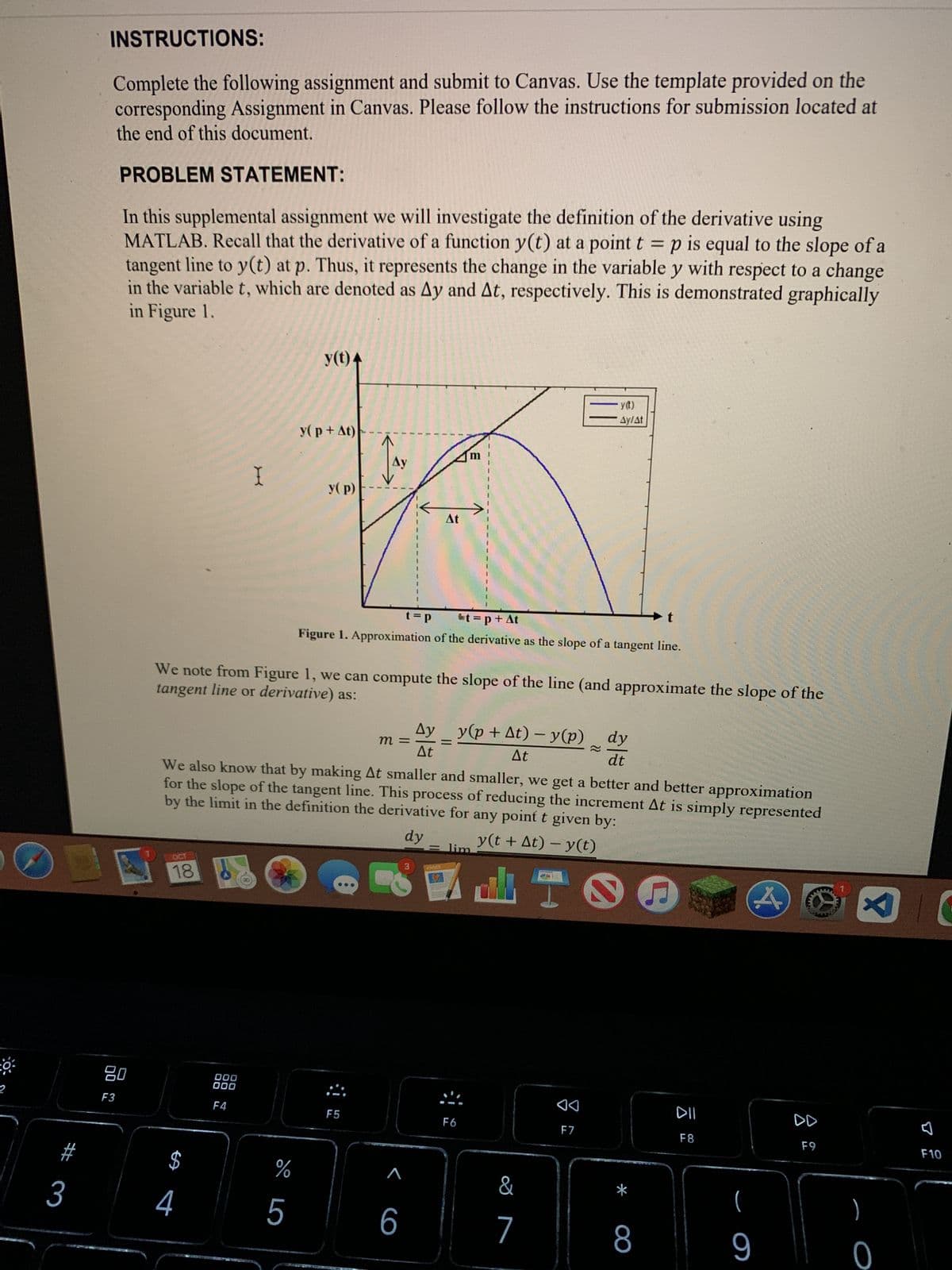
INSTRUCTIONS:
Complete the following assignment and submit to Canvas. Use the template provided on the
corresponding Assignment in Canvas. Please follow the instructions for submission located at
the end of this document.
PROBLEM STATEMENT:
In this supplemental assignment we will investigate the definition of the derivative using
MATLAB. Recall that the derivative of a function y(t) at a point t p is equal to the slope of a
tangent line to y(t) at p. Thus, it represents the change in the variable y with respect to a change
in the variable t, which are denoted as Ay and At, respectively. This is demonstrated graphically
in Figure 1.
80
F3
OCT
18
$
I
4
000
000
F4
y(t) 4
y( p + At)
%
5
y(p)
tangent line or derivative) as:
We note from Figure 1, we can compute the slope of the line (and approximate the slope of the
Ay
F5
t=p
t = p + At
Figure 1. Approximation of the derivative as the slope of a tangent line.
We also know that by making At smaller and smaller, we get a better and better approximation
for the slope of the tangent line. This process of reducing the increment At is simply represented
by the limit in the definition the derivative for any point t given by:
y(t + At) − y(t)
dy
m =
SC
At
6
3
Ay _ y(p+ At) — y(p)
=
At
At
- lim
y(t)
Ay/At
F6
&
7
F7
dy
dt
*
8
DII
F8
A
(
9
F9
www
)
0
3
F10
Transcribed Image Text:2 # 3 INSTRUCTIONS: Complete the following assignment and submit to Canvas. Use the template provided on the corresponding Assignment in Canvas. Please follow the instructions for submission located at the end of this document. PROBLEM STATEMENT: In this supplemental assignment we will investigate the definition of the derivative using MATLAB. Recall that the derivative of a function y(t) at a point t p is equal to the slope of a tangent line to y(t) at p. Thus, it represents the change in the variable y with respect to a change in the variable t, which are denoted as Ay and At, respectively. This is demonstrated graphically in Figure 1. 80 F3 OCT 18 $ I 4 000 000 F4 y(t) 4 y( p + At) % 5 y(p) tangent line or derivative) as: We note from Figure 1, we can compute the slope of the line (and approximate the slope of the Ay F5 t=p t = p + At Figure 1. Approximation of the derivative as the slope of a tangent line. We also know that by making At smaller and smaller, we get a better and better approximation for the slope of the tangent line. This process of reducing the increment At is simply represented by the limit in the definition the derivative for any point t given by: y(t + At) − y(t) dy m = SC At 6 3 Ay _ y(p+ At) — y(p) = At At - lim y(t) Ay/At F6 & 7 F7 dy dt * 8 DII F8 A ( 9 F9 www ) 0 3 F10
#
3
80
F3
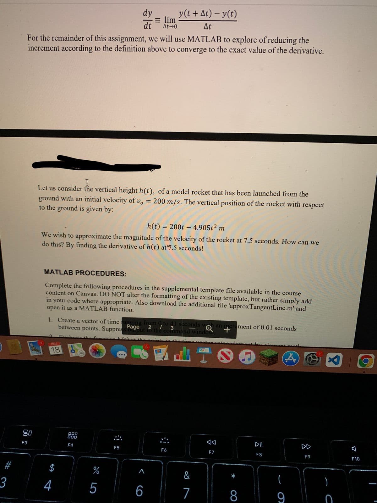
For the remainder of this assignment, we will use MATLAB to explore of reducing the
increment according to the definition above to converge to the exact value of the derivative.
I
Let us consider the vertical height h(t), of a model rocket that has been launched from the
ground with an initial velocity of vo = 200 m/s. The vertical position of the rocket with respect
to the ground is given by:
h(t) = 200t - 4.905t² m
We wish to approximate the magnitude of the velocity of the rocket at 7.5 seconds. How can we
do this? By finding the derivative of h(t) at 7.5 seconds!
MATLAB PROCEDURES:
Complete the following procedures in the supplemental template file available in the course
content on Canvas. DO NOT alter the formatting of the existing template, but rather simply add
in your code where appropriate. Also download the additional file 'approxTangentLine.m' and
open it as a MATLAB function.
OCT
18
1. Create a vector of time ranging from 0 to 41 seconds weh an increment of 0.01 seconds
between points. Suppress output to the command window
Page 2 1 3
+
ation hft) + 4h
$
dy
= lim
dt At-0
4
000
000
F4
%
5
F5
y(t + At) − y(t)
At
A
6
3
F6
&
7
◄◄
F7
8
DII
F8
A
(
9
DD
F9
XI
)
C
7
F10
Transcribed Image Text:# 3 80 F3 For the remainder of this assignment, we will use MATLAB to explore of reducing the increment according to the definition above to converge to the exact value of the derivative. I Let us consider the vertical height h(t), of a model rocket that has been launched from the ground with an initial velocity of vo = 200 m/s. The vertical position of the rocket with respect to the ground is given by: h(t) = 200t - 4.905t² m We wish to approximate the magnitude of the velocity of the rocket at 7.5 seconds. How can we do this? By finding the derivative of h(t) at 7.5 seconds! MATLAB PROCEDURES: Complete the following procedures in the supplemental template file available in the course content on Canvas. DO NOT alter the formatting of the existing template, but rather simply add in your code where appropriate. Also download the additional file 'approxTangentLine.m' and open it as a MATLAB function. OCT 18 1. Create a vector of time ranging from 0 to 41 seconds weh an increment of 0.01 seconds between points. Suppress output to the command window Page 2 1 3 + ation hft) + 4h $ dy = lim dt At-0 4 000 000 F4 % 5 F5 y(t + At) − y(t) At A 6 3 F6 & 7 ◄◄ F7 8 DII F8 A ( 9 DD F9 XI ) C 7 F10
Expert Solution
trending now

Trending now

This is a popular solution!

steps

Step by step

Solved in 2 steps with 2 images

Blurred answer
Recommended textbooks for you
Computer Networking: A Top-Down Approach (7th Edi…
Computer Engineering
ISBN:
9780133594140
Author:
James Kurose, Keith Ross
Publisher:
PEARSON
Computer Organization and Design MIPS Edition, Fi…
Computer Engineering
ISBN:
9780124077263
Author:
David A. Patterson, John L. Hennessy
Publisher:
Elsevier Science
Network+ Guide to Networks (MindTap Course List)
Computer Engineering
ISBN:
9781337569330
Author:
Jill West, Tamara Dean, Jean Andrews
Publisher:
Cengage Learning
Concepts of Database Management
Computer Engineering
ISBN:
9781337093422
Author:
Joy L. Starks, Philip J. Pratt, Mary Z. Last
Publisher:
Cengage Learning
Prelude to Programming
Computer Engineering
ISBN:
9780133750423
Author:
VENIT, Stewart
Publisher:
Pearson Education
Sc Business Data Communications and Networking, T…
Computer Engineering
ISBN:
9781119368830
Author:
FITZGERALD
Publisher:
WILEY