I am just looking for the solution of the theoritical part. I will take care of the portion that requires usage of Matlab software. 1.For the pendulum shown in Figure 1, write the equation ofmotion and use ode45 in MATLAB to integrate it. Additionally, com-pare your results for the angular velocity of the pendulum to that of thesmall angle approximation for (80, wn) = (20°, 0) and (60, wn) = (80°, 0).Additionally, let l = 1[m). For the submission you should include:(a) The equation of motion for the general, nonlinear case (this shouldbe an ordinary differential equation).(b) An expression for the angular velocity under the small angle spprox-imation. Note: The linearization of the small angle approximationwill allow you to derive the angular velocity as a function of timeanslytically (you should not use ode45 to solve this).(c) Two figures - one for esch set of initial conditions. Each figure shouldshow both angular velocities (nonlinear, and approximated) on thesame graph. 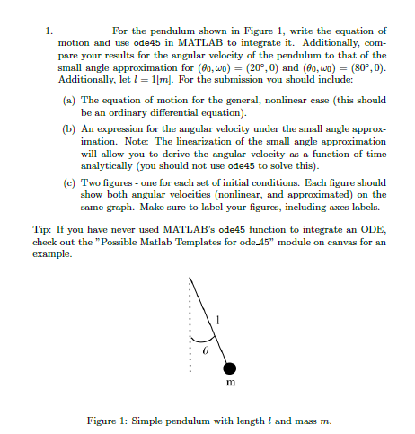Make sure to label your figures, including axes labels.Tip: If you have never used MATLAB's ode45 function to integrate an ODE,check out the "Possible Matlab Templates for ode.45" module on canvas for anexample.mFigure 1: Simple pendulum with length I and mass m.

The general equation of the pendulum can be derived by finding its Lagrangian. It is the easier way…

1. For the pendulum shown in Figure 1, write the cquation of motion and use ode45 in MATLAB to integrate it. Additionally, com- pare your results for the angular velocity of the pendulum to that of the small angle approximation for (00, wo) = (20°, 0) and (60, wo) = (80°, 0). Additionally, let l = 1[m). For the submission you should include: (m) The equation of motion for the general, nonlinear case (this should be an ordinary differential equation). (b) An expression for the angular velocity under the small angle approx- imation. Note: The linearization of the small angle approximation will allow you to derive the angular velocity as a function of time analytically (you should not use ode45 to solve this). (c) Two figures - one for ench set of initial conditions. Ench figure should show both angular velocities (nonlinear, and approximated) on the same graph. Make sure to label your figures, including axes labels. Tip: If you have never used MATLAB's ode45 function to integrate an ODE, check out the "Possible Matlab Templates for ode.45" module on canvas for an еxample. Figure 1: Simple pendulum with length I and mass m.

1. For the pendulum shown in Figure 1, write the cquation of motion and use ode45 in MATLAB to integrate it. Additionally, com- pare your results for the angular velocity of the pendulum to that of the small angle approximation for (00, wo) = (20°, 0) and (60, wo) = (80°, 0). Additionally, let l = 1[m). For the submission you should include: (m) The equation of motion for the general, nonlinear case (this should be an ordinary differential equation). (b) An expression for the angular velocity under the small angle approx- imation. Note: The linearization of the small angle approximation will allow you to derive the angular velocity as a function of time analytically (you should not use ode45 to solve this). (c) Two figures - one for ench set of initial conditions. Ench figure should show both angular velocities (nonlinear, and approximated) on the same graph. Make sure to label your figures, including axes labels. Tip: If you have never used MATLAB's ode45 function to integrate an ODE, check out the "Possible Matlab Templates for ode.45" module on canvas for an еxample. Figure 1: Simple pendulum with length I and mass m.