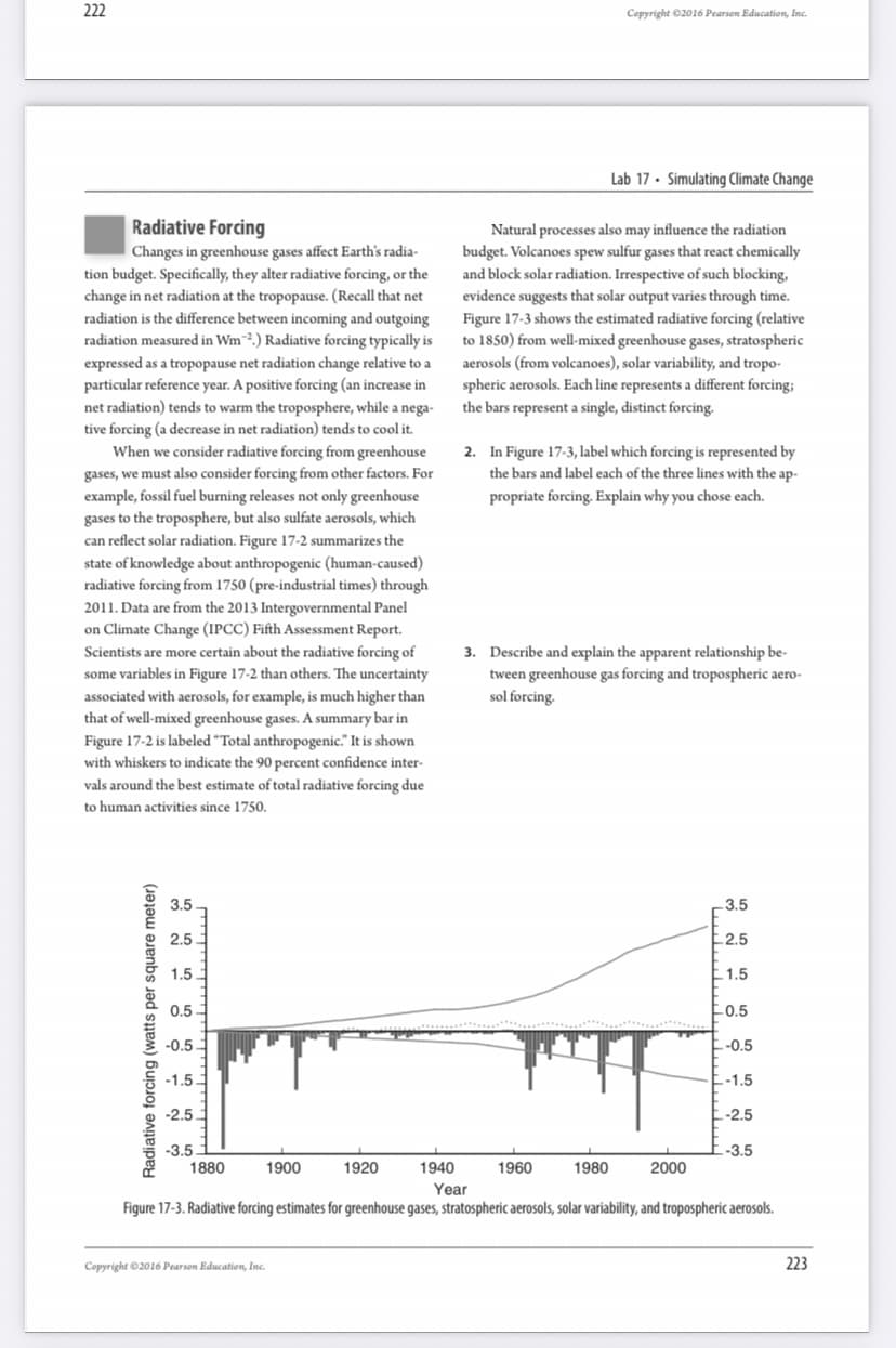
222Copyright @2016 Pearson Education, Inc.Lab 17 · Simulating Climate ChangeRadiative ForcingNatural processes also may influence the radiationbudget. Volcanoes spew sulfur gases that react chemicallyand block solar radiation. Irrespective of such blocking,evidence suggests that solar output varies through time.Figure 17-3 shows the estimated radiative forcing (relativeto 1850) from well-mixed greenhouse gases, stratosphericChanges in greenhouse gases affect Earth's radia-tion budget. Specifically, they alter radiative forcing, or thechange in net radiation at the tropopause. (Recall that netradiation is the difference between incoming and outgoingradiation measured in Wm².) Radiative forcing typically isexpressed as a tropopause net radiation change relative to aparticular reference year. A positive forcing (an increase innet radiation) tends to warm the troposphere, while a nega-tive forcing (a decrease in net radiation) tends to cool it.When we consider radiative forcing from greenhouseaerosols (from volcanoes), solar variability, and tropo-spheric aerosols. Each line represents a different forcing;the bars represent a single, distinct forcing.gases, we must also consider forcing from other factors. Forexample, fossil fuel burning releases not only greenhousegases to the troposphere, but also sulfate aerosols, whichcan reflect solar radiation. Figure 17-2 summarizes the2. In Figure 17-3, label which forcing is represented bythe bars and label each of the three lines with the ap-propriate forcing. Explain why you chose each.state of knowledge about anthropogenic (human-caused)radiative forcing from 1750 (pre-industrial times) through2011. Data are from the 2013 Intergovernmental Panelon Climate Change (IPCC) Fifth Assessment Report.3. Describe and explain the apparent relationship be-tween greenhouse gas forcing and tropospheric aero-sol forcing.Scientists are more certain about the radiative forcing ofsome variables in Figure 17-2 than others. The uncertaintyassociated with aerosols, for example, is much higher thanthat of well-mixed greenhouse gases. A summary bar inFigure 17-2 is labeled “Total anthropogenic." It is shownwith whiskers to indicate the 90 percent confidence inter-vals around the best estimate of total radiative forcing dueto human activities since 1750.3.53.52.5- 2.51.51.50.5-0.5-0.5.E-0.5-1.5-1.5-2.5.E-2.5-3.5-3.51880190019201940196019802000YearFigure 17-3. Radiative forcing estimates for greenhouse gases, stratospheric aerosols, solar variability, and tropospheric aerosols.Copyright 02016 Pearson Education, Inc.223Radiative forcing (watts per square meter) Name:Date:Lab17Simulating1/ Climate ChangeScan to view the Pre-Lab Videofor this lab.http://goo.gl/cv)NUIntroductionFew weather and climate topics currently generate more political debate than the issue ofhuman-induced, or anthropogenic, climate change. In this lab, we explore how humanactivities have influenced atmospheric greenhouse gas concentrations, and the methodsand challenges to linking such concentrations to historic and future climate change.ObjectivesAfter completing these exercises, you should be able to:Explain the historic link between greenhouse gas emissions, concentrations, radiativeforcing, and temperature changeApply the concept of feedbacks to specific examples of climate changeDescribe the range of temperature changes projected by climate models and theassumed emissions scenarios and climate sensitivity that produces these changesDescribe the correlation between ENSO events and average global temperatureEmissions and Concentrations1. IFCO, concentrations continued to increase at a ratePerhaps the least controversial part of this story isthat human activities release carbon dioxide (CO,) andother greenhouse gases, and that concentrations of CO,have steadily increased since regular measurement began in1958 (Figure 17-1). The rate of atmospheric CO, increaseof 2 ppm per year, what would be the approximateconcentration by the year 2050?exceeds that seen in the long-term ice core record and hasa chemical "fingerprint" that links it largely to the burningof fossil fuels. Further evidence shows that two possiblenatural sources of CO,-oceans and vegetation-actuallyhave taken up CO, during this period. Without this, atmo-spheric CO, concentrations would be even higher.Copyright ©2016 Pearson Education, Inc.221

The differential between inbound solar radiation and outbound terrestrial radiation is known as…

2. In Figure 17-3, label which forcing is represented by the bars and label each of the three lines with the ap- propriate forcing. Explain why you chose each. When we consider radiative forcing from greenhouse es, we must also consider forcing from other factors. For mple, fossil fuel burning releases not only greenhouse es to the troposphere, but also sulfate aerosols, which reflect solar radiation. Figure 17-2 summarizes the e of knowledge about anthropogenic (human-caused) ative forcing from 1750 (pre-industrial times) through 1. Data are from the 2013 Intergovernmental Panel Climate Change (IPCC) Fifth Assessment Report. entists are more certain about the radiative forcing of ne variables in Figure 17-2 than others. The uncertainty ociated with aerosols, for example, is much higher than t of well-mixed greenhouse gases. A summary bar in ure 17-2 is labeled "Total anthropogenic." It is shown h whiskers to indicate the 90 percent confidence inter- around the best estimate of total radiative forcing due muman activities since 1750. 3. Describe and explain the apparent relationship be- tween greenhouse gas forcing and tropospheric aero- sol forcing. 3.5 3.5 2.5 2.5 1.5. E1.5 0.5- E0.5 -0.5. E-0.5 -1.5. E-1.5 -2.5. E-2.5 -3.5. 1880 -3.5 1900 1920 1940 1960 1980 2000 Year Figure 17-3. Radiative forcing estimates for greenhouse gases, stratospheric aerosols, solar variability, and tropospheric aerosols. Radiative forcing (watts per square meter)

9th Edition

ISBN:9780134746241

Author:Edward J. Tarbuck, Frederick K. Lutgens, Dennis G. Tasa

Publisher:Edward J. Tarbuck, Frederick K. Lutgens, Dennis G. Tasa

Chapter1: The Study Of Minerals

Section: Chapter Questions

Problem 1LR