(c) No accidents (d) Fewer than five accidents lity Distributions 4.4.4 In a study of the effectiveness of an insecticide against a certain insect, a large area of land was sprayed. Later the area was examined for live insects by randomly selecting squares and counting the number of live insects per square. Past experience has shown the average number of live insects per square after spraying to be .5. If the number of live insects per square follows a Poisson distribution, find the probability that a selected 10 square will contain: (a) Exactly one live insect (b) No live insects (c) Exactly four live insects (d) One or more live insects 46 The No 4.5 Continuous Probability Distributions The probability distributions considered thus far, the binomial and the Poisson, are distributions of discrete variables. Let us now consider distributions of continuous random variables. In Chapter 1, we stated that a continuous variable is one that can assume any value within a specified interval of values assumed by the variable. Consequently, between any two values assumed by a continuous variable, there exist an infinite number of values. To help us understand the nature of the distribution of a continuous random variable, let us consider the data presented in Table 1.4.1 and Figure 2.6.1. In the table, we have 189 values of the random variable, age. The histogram of Figure 2.6.1 was constructed by locating speceilicd Poms on a line representing the measurement of interest and erecting a series of rectangies. whose widths were the distances between two specified points on the line, and whose heights represented the number of values of the variable falling between the two specified points. The intervals defined by any two consecutive specified points we called class intervals. As was noted of the variable between the horizontal scale boundaries of these subareas. This provides a way be calculated: merely determine the proportion of the histogram's total area falling between the whereby the relative frequency of occurrence of values between any two specified points can specified points. This can be done more conveniently by consulting the relative frequency or cumulative relative frequency columns of Table 2.3.2. and the width of our class intervals is made very small. The resulting histogram could look like Imagine now the situation where the number of values of our random variable is very large that shown in Figure 4.5.1. frequency polygon, clearly we would have a much smoother figure than the frequency polygon If we were to connect the midpoints of the cells of the histogram in Figure 4.5.1 to form a In general, as the number of observations, n, approaches infinity, and the width of the class Figure 4.5.2. Such smooth curves are used to represent graphically the distributions of continuous intervals approaches zero, the frequency polygon approaches a smooth curve such as is shown in Consequences when we deal with probability distri- as was true with the histogram, and ints on the r-axis is equal to cd at the two points m variable is area
(c) No accidents (d) Fewer than five accidents lity Distributions 4.4.4 In a study of the effectiveness of an insecticide against a certain insect, a large area of land was sprayed. Later the area was examined for live insects by randomly selecting squares and counting the number of live insects per square. Past experience has shown the average number of live insects per square after spraying to be .5. If the number of live insects per square follows a Poisson distribution, find the probability that a selected 10 square will contain: (a) Exactly one live insect (b) No live insects (c) Exactly four live insects (d) One or more live insects 46 The No 4.5 Continuous Probability Distributions The probability distributions considered thus far, the binomial and the Poisson, are distributions of discrete variables. Let us now consider distributions of continuous random variables. In Chapter 1, we stated that a continuous variable is one that can assume any value within a specified interval of values assumed by the variable. Consequently, between any two values assumed by a continuous variable, there exist an infinite number of values. To help us understand the nature of the distribution of a continuous random variable, let us consider the data presented in Table 1.4.1 and Figure 2.6.1. In the table, we have 189 values of the random variable, age. The histogram of Figure 2.6.1 was constructed by locating speceilicd Poms on a line representing the measurement of interest and erecting a series of rectangies. whose widths were the distances between two specified points on the line, and whose heights represented the number of values of the variable falling between the two specified points. The intervals defined by any two consecutive specified points we called class intervals. As was noted of the variable between the horizontal scale boundaries of these subareas. This provides a way be calculated: merely determine the proportion of the histogram's total area falling between the whereby the relative frequency of occurrence of values between any two specified points can specified points. This can be done more conveniently by consulting the relative frequency or cumulative relative frequency columns of Table 2.3.2. and the width of our class intervals is made very small. The resulting histogram could look like Imagine now the situation where the number of values of our random variable is very large that shown in Figure 4.5.1. frequency polygon, clearly we would have a much smoother figure than the frequency polygon If we were to connect the midpoints of the cells of the histogram in Figure 4.5.1 to form a In general, as the number of observations, n, approaches infinity, and the width of the class Figure 4.5.2. Such smooth curves are used to represent graphically the distributions of continuous intervals approaches zero, the frequency polygon approaches a smooth curve such as is shown in Consequences when we deal with probability distri- as was true with the histogram, and ints on the r-axis is equal to cd at the two points m variable is area

MATLAB: An Introduction with Applications
6th Edition
ISBN:9781119256830
Author:Amos Gilat
Publisher:Amos Gilat
Chapter1: Starting With Matlab
Section: Chapter Questions
Problem 1P

Related questions
Question
please help with 4.4.4 "d" only
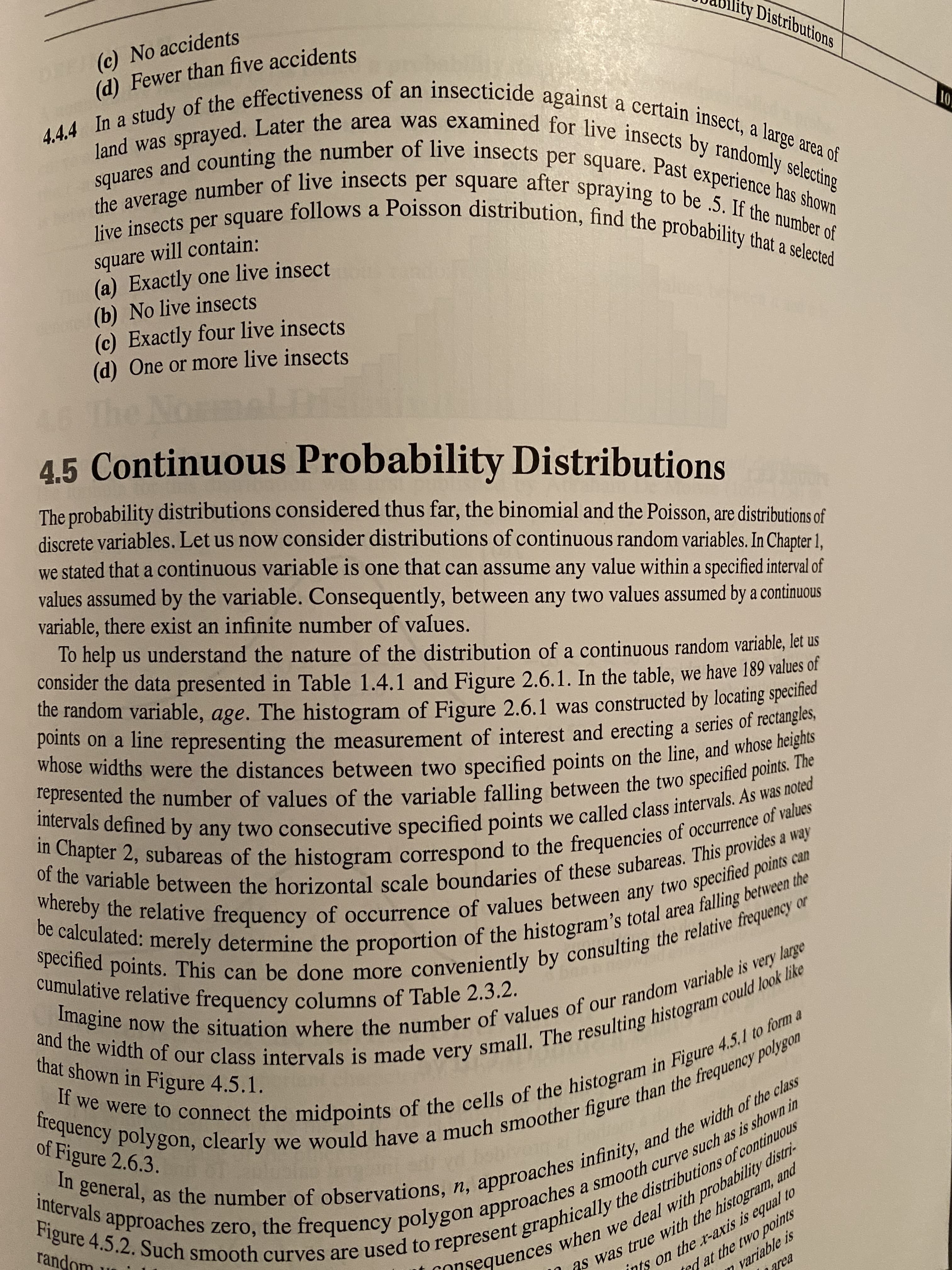
Transcribed Image Text:(c) No accidents
(d) Fewer than five accidents
lity Distributions
4.4.4 In a study of the effectiveness of an insecticide against a certain insect, a large area of
land was sprayed. Later the area was examined for live insects by randomly selecting
squares and counting the number of live insects per square. Past experience has shown
the average number of live insects per square after spraying to be .5. If the number of
live insects per square follows a Poisson distribution, find the probability that a selected
10
square will contain:
(a) Exactly one live insect
(b) No live insects
(c) Exactly four live insects
(d) One or more live insects
46 The No
4.5 Continuous Probability Distributions
The probability distributions considered thus far, the binomial and the Poisson, are distributions of
discrete variables. Let us now consider distributions of continuous random variables. In Chapter 1,
we stated that a continuous variable is one that can assume any value within a specified interval of
values assumed by the variable. Consequently, between any two values assumed by a continuous
variable, there exist an infinite number of values.
To help us understand the nature of the distribution of a continuous random variable, let us
consider the data presented in Table 1.4.1 and Figure 2.6.1. In the table, we have 189 values of
the random variable, age. The histogram of Figure 2.6.1 was constructed by locating speceilicd
Poms on a line representing the measurement of interest and erecting a series of rectangies.
whose widths were the distances between two specified points on the line, and whose heights
represented the number of values of the variable falling between the two specified points. The
intervals defined by any two consecutive specified points we called class intervals. As was noted
of the variable between the horizontal scale boundaries of these subareas. This provides a way
be calculated: merely determine the proportion of the histogram's total area falling between the
whereby the relative frequency of occurrence of values between any two specified points can
specified points. This can be done more conveniently by consulting the relative frequency or
cumulative relative frequency columns of Table 2.3.2.
and the width of our class intervals is made very small. The resulting histogram could look like
Imagine now the situation where the number of values of our random variable is very large
that shown in Figure 4.5.1.
frequency polygon, clearly we would have a much smoother figure than the frequency polygon
If we were to connect the midpoints of the cells of the histogram in Figure 4.5.1 to form a
In general, as the number of observations, n, approaches infinity, and the width of the class
Figure 4.5.2. Such smooth curves are used to represent graphically the distributions of continuous
intervals approaches zero, the frequency polygon approaches a smooth curve such as is shown in
Consequences when we deal with probability distri-
as was true with the histogram, and
ints on the r-axis is equal to
cd at the two points
m variable is
area
Expert Solution
This question has been solved!
Explore an expertly crafted, step-by-step solution for a thorough understanding of key concepts.

This is a popular solution!

Trending now
This is a popular solution!

Step by step
Solved in 2 steps with 2 images

Knowledge Booster


Learn more about
Need a deep-dive on the concept behind this application? Look no further. Learn more about this topic, statistics and related others by exploring similar questions and additional content below.Recommended textbooks for you
MATLAB: An Introduction with Applications
Statistics
ISBN:
9781119256830
Author:
Amos Gilat
Publisher:
John Wiley & Sons Inc

Probability and Statistics for Engineering and th…
Statistics
ISBN:
9781305251809
Author:
Jay L. Devore
Publisher:
Cengage Learning

Statistics for The Behavioral Sciences (MindTap C…
Statistics
ISBN:
9781305504912
Author:
Frederick J Gravetter, Larry B. Wallnau
Publisher:
Cengage Learning
MATLAB: An Introduction with Applications
Statistics
ISBN:
9781119256830
Author:
Amos Gilat
Publisher:
John Wiley & Sons Inc
Probability and Statistics for Engineering and th…
Statistics
ISBN:
9781305251809
Author:
Jay L. Devore
Publisher:
Cengage Learning
Statistics for The Behavioral Sciences (MindTap C…
Statistics
ISBN:
9781305504912
Author:
Frederick J Gravetter, Larry B. Wallnau
Publisher:
Cengage Learning

Elementary Statistics: Picturing the World (7th E…
Statistics
ISBN:
9780134683416
Author:
Ron Larson, Betsy Farber
Publisher:
PEARSON

The Basic Practice of Statistics
Statistics
ISBN:
9781319042578
Author:
David S. Moore, William I. Notz, Michael A. Fligner
Publisher:
W. H. Freeman

Introduction to the Practice of Statistics
Statistics
ISBN:
9781319013387
Author:
David S. Moore, George P. McCabe, Bruce A. Craig
Publisher:
W. H. Freeman