Can you please annotate the two images attached. Also send a picture of the parts where you annotated/highlighted please I would really appreciate it I really need it is very important
Can you please annotate the two images attached. Also send a picture of the parts where you annotated/highlighted please I would really appreciate it I really need it is very important

Concepts of Biology
1st Edition
ISBN:9781938168116
Author:Samantha Fowler, Rebecca Roush, James Wise
Publisher:Samantha Fowler, Rebecca Roush, James Wise
Chapter10: Biotechnology
Section: Chapter Questions
Problem 13CTQ: Identify a possible advantage and a possible disadvantage of a genetic test that would identify...

Related questions

Question
Can you please annotate the two images attached. Also send a picture of the parts where you annotated/highlighted please I would really appreciate it
I really need it is very important
Transcribed Image Text:beetle eggs were influenced by temperature (F= 70083; df = 4.
1891; P = 0.0001). There was a significant decrease in the number
of days required for egg development from 20°C to 35°C, and a
significant increase at 38°C (P = 0.05; Tukey's test).
Larval development times were influenced by temperature
(F= 9999; df = 4, 3519; P=0.0001). These development times.
were significantly greatest at 20°C and lowest at 35°C. Pupal de-
velopment times also were influenced by temperature (F = 5986;
df = 4, 3178; P = 0.0001). These development times significantly
decreased from 20°C to 35°C, but there was no further significant.
decrease at 38°C. There was a significant decrease in the number
of days required for immature development (egg hatch to adult
emergence) and total development (oviposition to adult emergence)
from 20°C to 35°C, and a significant increase at 38°C (P = 0.05:
Tukey's test). Therefore there was ample evidence of high
temperature inhibition of development.
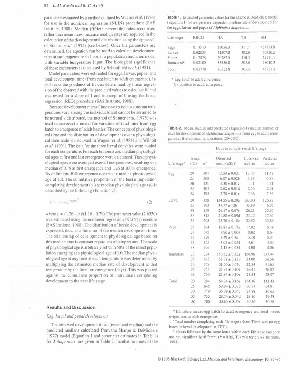
Density effect on development
Larval development times were significantly lower at density
of 1 larva per gram than at densities of 3 or 6 larvae per gram
at 30°C to 38°C, but not at 20°C and 25°C when analysed
separately by temperature. No significant differences in larval
development occurred between 3 and 6 larvae per gram at any
of the temperature (P = 0.05; Tukey's test) (Fig. 1) Pupal
development times were not influenced by the density levels of
larvae preceding pupation.
DEVELOPMENTAL TIME (DAYS)
140
120
100
80-
60-
40
20
25
1 LARVA PER G
3 LARVAE PER G
B6 LARVAE PER G
30 35
TEMPERATURE C
38
Fig. 1. Mean number of days for larval development of Alphitobius
diaperinus reared at three densities (1, 3 and 6 larvae per gram of
medium) at each of five constant temperatures (°C).
Developmental functions.
The temperature-dependent median development rates of
A.diaperinus were well described by the Sharpe & DeMichele
model (Equation 1) incorporating high temperature inhibition
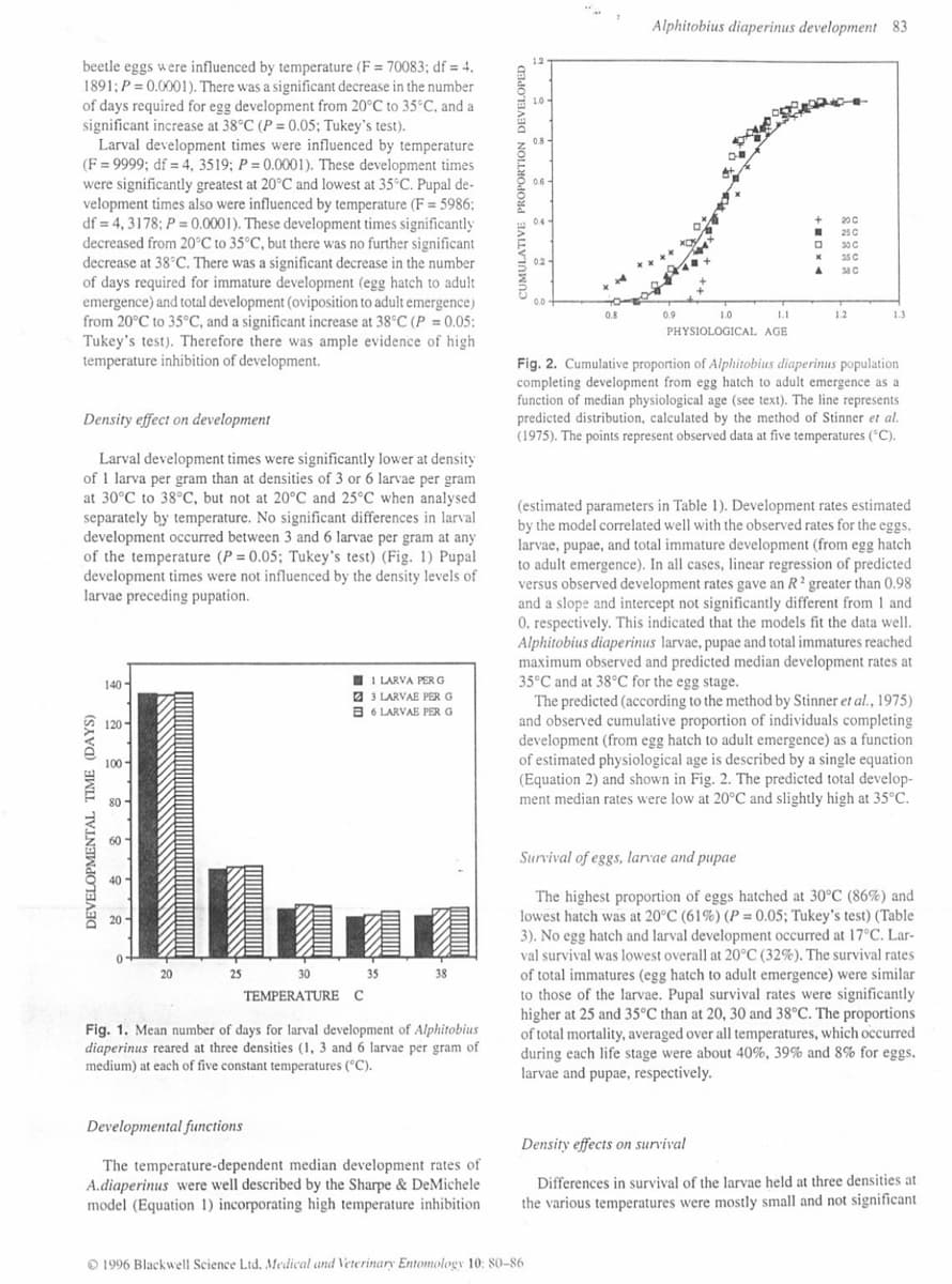
CUMULATIVE PROPORTION DEVELOPED
1.0
0.8
0.6
0.4
1996 Blackwell Science Ltd. Medical and Veterinary Entomology 10: 80-86
02
0.0
0.8
Alphitobius diaperinus development 83
1.0
1.1
PHYSIOLOGICAL AGE
0.9
+ DX4
25 C
30 C
35 C
A 38 C
1.2
1.3
Fig. 2. Cumulative proportion of Alphitobius diaperinus population
completing development from egg hatch to adult emergence as a
function of median physiological age (see text). The line represents
predicted distribution, calculated by the method of Stinner et al.
(1975). The points represent observed data at five temperatures (°C).
(estimated parameters in Table 1). Development rates estimated
by the model correlated well with the observed rates for the eggs,
larvae, pupae, and total immature development (from egg hatch
to adult emergence). In all cases, linear regression of predicted
versus observed development rates gave an R2 greater than 0.98
and a slope and intercept not significantly different from 1 and
0, respectively. This indicated that the models fit the data well.
Alphitobius diaperinus larvae, pupae and total immatures reached
maximum observed and predicted median development rates at
35°C and at 38°C for the egg stage.
The predicted (according to the method by Stinner et al., 1975)
and observed cumulative proportion of individuals completing
development (from egg hatch to adult emergence) as a function
of estimated physiological age is described by a single equation
(Equation 2) and shown in Fig. 2. The predicted total develop-
ment median rates were low at 20°C and slightly high at 35°C.
Survival of eggs, larvae and pupae
The highest proportion of eggs hatched at 30°C (86%) and
lowest hatch was at 20°C (61%) ( P = 0.05; Tukey's test) (Table
3). No egg hatch and larval development occurred at 17°C. Lar-
val survival was lowest overall at 20°C (32 %). The survival rates
of total immatures (egg hatch to adult emergence) were similar
to those of the larvae. Pupal survival rates were significantly
higher at 25 and 35°C than at 20, 30 and 38°C. The proportions
of total mortality, averaged over all temperatures, which occurred
during each life stage were about 40%, 39% and 8% for eggs.
larvae and pupae, respectively.
Density effects on survival
Differences in survival of the larvae held at three densities at
the various temperatures were mostly small and not significant
Transcribed Image Text:82 L. M. Rueda and R. C. Axtell
parameters estimated by a method outlined by Wagner et al. (1984)
for use in the nonlinear regression (NLIN) procedure (SAS
Institute, 1988). Median (fiftieth percentile) rates were used
rather than mean rates, because median rates are required in the
calculation of the developmental distribution using the approach
of Stinner et al. (1975) (see below). Once the parameters are
determined, the equation can be used to calculate development
rates at any temperature and used in a population simulation model
with variable temperature input. The biological significance
of these parameters is discussed by Schoolfield et al. (1981).
Model parameters were estimated for eggs, larvae, pupae, and
total development time (from egg hatch to adult emergence). In
each case the goodness of fit was determined by linear regres-
sion of the observed with the predicted values to calculate R² and
was tested for a slope of 1 and intercept of 0 using the linear
regression (REG) procedure (SAS Institute, 1988).
Because development rates of insects exposed to constant tem-
peratures vary among the individuals and cannot be assumed to
be normally distributed, the method of Stinner et al. (1975) was
used to construct a model for variation of total time from egg
hatch to emergence of adult beetles. The concepts of physiologi-
cal time and the distribution of development over a physiologi-
cal time scale is discussed in Wagner et al. (1984) and Wilhoit
et al. (1991). The data for the three larval densities were pooled
for each temperature. For each temperature, median physiologi-
cal ages at first and last emergence were calculated. These physi-
ological ages were averaged over all temperatures, resulting in a
median of 0.79 at first emergence and 1.26 at 100% emergence.
By definition. 50% emergence occurs at a median physiological
age of 1.0. The cumulative proportion of the beetle population
completing development (y) at median physiological age (p) is
described by the following (Equation 2):
y = (1-²6350²
(2)
where z = (1.26-p)/(1.26-0.79). The parameter value (2.6350)
was estimated using the nonlinear regression (NLIN) procedure
(SAS Institute, 1988). The distribution of beetle development is
expressed, thus, as a function of the median development time.
The relationship of development to physiological age based on
this median time is constant regardless of temperature. The scale
of physiological age is arbitrarily set with 50% of the insect popu-
lation emerging at a physiological age of 1.0. The median physi-
ological age at any time at each temperature was determined by
multiplying the estimated median rate of development at that
temperature by the time for emergence (days). This was plotted
against the cumulative proportion of individuals completing
development to the next life stage.
Results and Discussion
Egg, larval and pupal development
The observed development times (mean and median) and the
predicted medians calculated from the Sharpe & DeMichele
(1977) model (Equation 1 and parameter estimates in Table 1)
for A.diaperinus are given in Table 2. Incubation times of the
Table 1. Estimated parameter values for the Sharpe & DeMichele model
(Equation 1) for temperature-dependent median rate of development for
the eggs, larvae and pupae of Alphitobus diaperinus.
Life stage
HA
ΤΗ
17056.3
311.7
ni
41307.8
Eggs
Larvae
Pupae
Immature*
302.0
20787.5
310.3
35556.8
303.6
Total
30522.8
305.5
Egg hatch to adult emergence.
Oviposition to adult emergence.
Larva
RH025
Temp.
Life stage (FC)
Egg
Pupa
0.14540
0.02833
0.12078
0.02180
0.01778
Table 2. Mean. median and predicted (Equation 1) median number of
days for development of Alphitobius diaperinus from egg to adult emer-
gence at five constant temperatures (20-38°C).
Immature
Total
20
25
30
35
38
20
25
30
35
38
20
25
30
35
38
294
645
779
755
706
294
645
779
755
706
294
645
779
35 755
38 706
20
25
30
20
25
n'
30
35
38
304
360
431
404
393
358
693
859
815
795
13.59 ± 0.02a
6.07 ± 0.02b
4.38±0.01c
2.62 ± 0.01d
2.70 ± 0.01e
Days to complete each life stage
Observed
mean (SE):
13.40
5.99
4.41
Observed Predicted
median median
2.56
2.56
134.55 ± 0.29a
45.77 + 12b
26.17 ± 0.07c
26.21
21.88 0.09d 22.42
23.76±0.10e 23.92
133.00
45.99
HH
16.810.17a 17.02
7.96±0.06b 8.02
424754.8
50930.5
47111.4
48019.3
45727.3
5.49±0.3c 5.48
4.03±0.03d 4.01
4.12 0.03d 4.08
150.62±0.32a 150.96
53.78 0.13b 54.00
31.66 ± 0.07c 32.34
25.94±0.10d 26.41
27.84 ± 0.10e 28.54
164.240.16a 164.36
59.94±0.07b 60.17
36.08 ± 0.04c 37.88
28.74 +0.04d 28.96
30.65±0.05e 30.76
11.43
6.88
4.21
2.61
2.56
126.89
46.93
25.95
22.62
23.80
15.49
8.64
5.31
4.05
4.06
137.44
56.56
31.65
26.82
28.27
143.43
64.91
36.65
29.49
30.50
* Immature means egg hatch to adult emergence and total means
oviposition to adult emergence.
*Total number completing each file stage (Note: There was no egg
hatch or larval development at 17°C). .
Means followed by the same letter within each life stage category
are not significantly different (P=0.05, Tukey's test: SAS Institute,
1988).
1996 Blackwell Science Ltd, Medical and Veterinary Entomology 10: 80-86
Expert Solution
This question has been solved!
Explore an expertly crafted, step-by-step solution for a thorough understanding of key concepts.

Step by step
Solved in 3 steps with 2 images

Knowledge Booster


Learn more about
Need a deep-dive on the concept behind this application? Look no further. Learn more about this topic, biology and related others by exploring similar questions and additional content below.Recommended textbooks for you
Concepts of Biology
Biology
ISBN:
9781938168116
Author:
Samantha Fowler, Rebecca Roush, James Wise
Publisher:
OpenStax College
Concepts of Biology
Biology
ISBN:
9781938168116
Author:
Samantha Fowler, Rebecca Roush, James Wise
Publisher:
OpenStax College