Home Insert Page Layout Formulas Data Review View A B Purchasing Department Costs Dollar Value of Merchandise Purchased Number of Purchase Number of Suppliers (No. of Ss) Orders (PDC) $1,522,000 Department Store (MP$) $ 68,307,000 (No. of POs) 4,345 Baltimore 125 230 Chicago Los Angeles 1,095,000 33,463,000 2,548 542,000 121,800,000 1,420 8 4 2,053,000 Miami 119,450,000 5,935 188 5 33,575,000 New York 1,068,000 2,786 21 Phoenix 517,000 29,836,000 1,334 29 1,544,000 1,761,000 Seattle 102,840,000 38,725,000 7,581 101 St. Louis 3,623 127 Toronto 1,605,000 139,300,000 1,712 202 10 1,263,000 130,110,000 Vancouver 4,736 196 11 2. 3. 6. Regression 1: PDC = a + (b × MPS) Variable Coefficient Standard Error t-Value Constant $1,041,421 $346,709 3.00 Independent variable 1: MPS 0.0031 0.0038 0.83 p2 = 0.08; Durbin-Watson statistic = 2.41 Regression 2: PDc = a + (b x No. of POs) Variable Standard Error Coefficient t-Value Constant S722,538 $265,835 2.72 Independent variable 1: No. of POs 64.84 159.48 2.46 p2 = 0.43; Durbin-Watson statistic 1.97 Regression 3. PDC = a + (b × No. of Ss) Variable Coefficient Standard Error t-Value Constant $828,814 $246,571 3.36 $ 3,816 $ 1,698 Independent variable 1: No. of Ss 2.25 p? = 0.39; Durbin-Watson statistic 2.01


Process Costing
Process costing is a sort of operation costing which is employed to determine the value of a product at each process or stage of producing process, applicable where goods produced from a series of continuous operations or procedure.
Job Costing
Job costing is adhesive costs of each and every job involved in the production processes. It is an accounting measure. It is a method which determines the cost of specific jobs, which are performed according to the consumer’s specifications. Job costing is possible only in businesses where the production is done as per the customer’s requirement. For example, some customers order to manufacture furniture as per their needs.
ABC Costing
Cost Accounting is a form of managerial accounting that helps the company in assessing the total variable cost so as to compute the cost of production. Cost accounting is generally used by the management so as to ensure better decision-making. In comparison to financial accounting, cost accounting has to follow a set standard ad can be used flexibly by the management as per their needs. The types of Cost Accounting include – Lean Accounting, Standard Costing, Marginal Costing and Activity Based Costing.
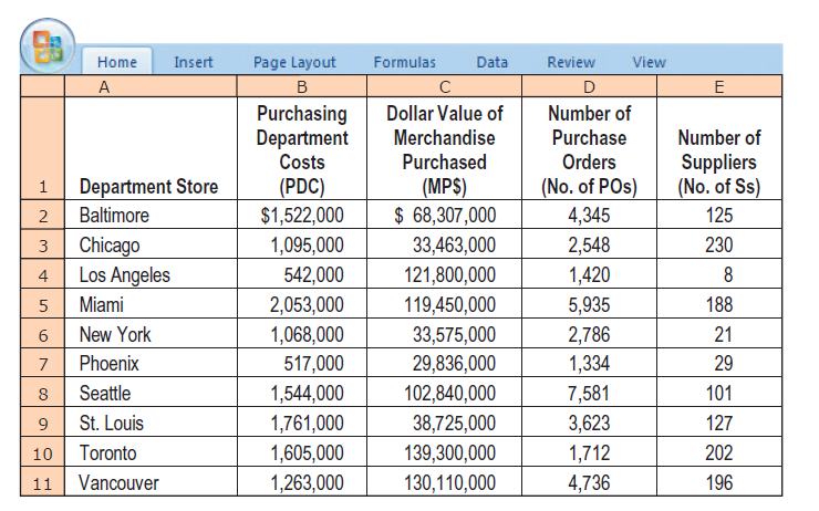
Purchasing department cost drivers, activity-based costing, simple regression analysis. Perfect Fit operates a chain of 10 retail department stores. Each department store makes its own purchasing decisions. Carl Hart, assistant to the president of Perfect Fit, is interested in better understanding the drivers of purchasing department costs. For many years, Perfect Fit has allocated purchasing department costs to products on the basis of the dollar value of merchandise purchased. A $100 item is allocated 10 times as many overhead costs associated with the purchasing department as a $10 item.
Hart recently attended a seminar titled “Cost Drivers in the Retail Industry.” In a presentation at the seminar, Kaliko Fabrics, a leading competitor that has implemented activity-based costing, reported number of purchase orders and number of suppliers to be the two most important cost drivers of purchasing department costs. The dollar value of merchandise purchased in each purchase order was not found to be a significant cost driver. Hart interviewed several members of the purchasing department at the Perfect Fit store in Miami. They believed that Kaliko Fabrics’ conclusions also applied to their purchasing department. Hart collects the following data for the most recent year for Perfect Fit’s 10 retail department stores:
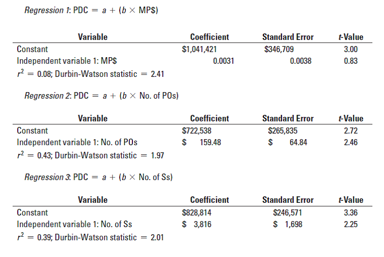
Hart decides to use simple regression analysis to examine whether one or more of three variables (the last three columns in the table) are cost drivers of purchasing department costs. Summary results for these regressions are as follows:
- Compare and evaluate the three simple regression models estimated by Hart. Graph each one. Also, use the format employed in Exhibit 10-18 (page 406) to evaluate the information.
- Do the regression results support the Kaliko Fabrics’ presentation about the purchasing department’s cost drivers? Which of these cost drivers would you recommend in designing an ABC system?
- How might Hart gain additional evidence on drivers of purchasing department costs at each of Perfect Fit’s stores?


Trending now
This is a popular solution!

Step by step
Solved in 10 steps with 8 images


