See the photo for the examples. A. Determine the area BELOW the following: 1. z = 3.1 2. z = 1.67 3. z = 0.76 B. Determine the area ABOVE the following: 1. z = -2.5 2. z = 1.96 3. z = -0.15 C. Determine the area of the region indicated: 1. -1 < z < 1 2. -1.5 < z < 2.5 3. -2.33 < z < 1.64
See the photo for the examples. A. Determine the area BELOW the following: 1. z = 3.1 2. z = 1.67 3. z = 0.76 B. Determine the area ABOVE the following: 1. z = -2.5 2. z = 1.96 3. z = -0.15 C. Determine the area of the region indicated: 1. -1 < z < 1 2. -1.5 < z < 2.5 3. -2.33 < z < 1.64

MATLAB: An Introduction with Applications
6th Edition
ISBN:9781119256830
Author:Amos Gilat
Publisher:Amos Gilat
Chapter1: Starting With Matlab
Section: Chapter Questions
Problem 1P

Related questions

Question
See the photo for the examples.
A. Determine the area BELOW the following:
1. z = 3.1
2. z = 1.67
3. z = 0.76
B. Determine the area ABOVE the following:
1. z = -2.5
2. z = 1.96
3. z = -0.15
C. Determine the area of the region indicated:
1. -1 < z < 1
2. -1.5 < z < 2.5
3. -2.33 < z < 1.64
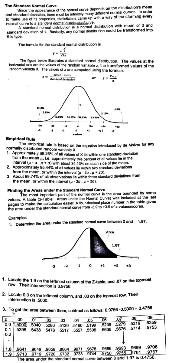
Transcribed Image Text:The Standard Normal Curve
Since the appearance of the normal curve depends on the distribution's mean
and standard deviation, there must be infinitely many different normal curves. In order
to make use of its properties, statisticians came up with a way of transforming every
normal curve to a standard normal distribution/curve.
A standard normal distribution is a normal distribution with mean of 0 and
standard deviation of 1. Basically, any normal distribution could be transformed into
this type.
The formula for the standard normal distribution is
y = an
The figure below illustrates a standard normal distribution. The values at the
horizontal axis are the values of the random variable z, the transformed values of the
random variable X. The values of z are computed using the formula:
value - mean
or z= X-4
standard deviation
0.13%
13%
2.19%
2.13%
13.50% 34.1% 34.13
13.59%
30
-20
-lo
lo
+20
+30
-2
-1
+1
vahues
Empirical Rule
The empirical rule is based on the equation introduced by de Moivre for any
normally distributed random variable X.
1. Approximately 68.26% of all values of X lie within one standard deviation
from the mean u, i.e. approximately this percent of all values lie in the
interval (u - o, u + o) with about 34.13% on each side of the mean.
2. Approximately 95.44% of all values lie within two standard deviations
from the mean, or within the interval (u - 20 , u + 20).
3.
About 99.74% of all observations lie within three standard deviations from
the mean, or within the interval (u - 30 , u+ 30).
Finding the Areas under the Standard Normal Curve
The most important part of the normal curve is the area bounded by some
values. A table (z-Table: Areas under the Normal Curve) was included at the last
pages to make the calculation easier. A four-decimal-place number in the table gives
the area under the standard normal curve from -3.9 to +3.9 of z-values/scores.
Examples
1. Determine the area under the standard normal curve between 0 and 1.97.
Area
1.97
-1 0 +1 +2
-3
-2
1. Locate the 1.9 on the leftmost column of the Z-table, and .07 on the topmost
row. Their intersection is 0.9756.
2. Locate 0.0 on the leftmost column, and .00 on the topmost row. Their
intersection is .5000.
%3D
3. To get the area between them, subtract as follows: 0.9756 -0.5000 = 0.4756
.02
.07 .08
.09
.00
.01
.03
.04 .05
.06
0.0 L5000 .5040 .5080 5120 5160 5199 5239 .5279 .5319 .5359
0.1
.5398 .5438 .5478 .5517 .5557 .5596 .5636 .5675 .5714 .5753
0.2
1.8 .9641 .9649 .9656 .9664 9671 .9678 .9686 .9693 .9699 .9706
1.9 | .9713 .9719 .9726 .9732 .9738 .9744 9750 9156 9761 .9767
The area under the standard normal curve between 0 and 1.97 is 0.4756.
Expert Solution
This question has been solved!
Explore an expertly crafted, step-by-step solution for a thorough understanding of key concepts.

This is a popular solution!

Trending now
This is a popular solution!

Step by step
Solved in 3 steps with 9 images

Knowledge Booster


Learn more about
Need a deep-dive on the concept behind this application? Look no further. Learn more about this topic, statistics and related others by exploring similar questions and additional content below.Recommended textbooks for you
MATLAB: An Introduction with Applications
Statistics
ISBN:
9781119256830
Author:
Amos Gilat
Publisher:
John Wiley & Sons Inc

Probability and Statistics for Engineering and th…
Statistics
ISBN:
9781305251809
Author:
Jay L. Devore
Publisher:
Cengage Learning

Statistics for The Behavioral Sciences (MindTap C…
Statistics
ISBN:
9781305504912
Author:
Frederick J Gravetter, Larry B. Wallnau
Publisher:
Cengage Learning
MATLAB: An Introduction with Applications
Statistics
ISBN:
9781119256830
Author:
Amos Gilat
Publisher:
John Wiley & Sons Inc
Probability and Statistics for Engineering and th…
Statistics
ISBN:
9781305251809
Author:
Jay L. Devore
Publisher:
Cengage Learning
Statistics for The Behavioral Sciences (MindTap C…
Statistics
ISBN:
9781305504912
Author:
Frederick J Gravetter, Larry B. Wallnau
Publisher:
Cengage Learning

Elementary Statistics: Picturing the World (7th E…
Statistics
ISBN:
9780134683416
Author:
Ron Larson, Betsy Farber
Publisher:
PEARSON

The Basic Practice of Statistics
Statistics
ISBN:
9781319042578
Author:
David S. Moore, William I. Notz, Michael A. Fligner
Publisher:
W. H. Freeman

Introduction to the Practice of Statistics
Statistics
ISBN:
9781319013387
Author:
David S. Moore, George P. McCabe, Bruce A. Craig
Publisher:
W. H. Freeman