
Concept explainers
Videos
a.
Construct a time series plot for temperature using the given data.
Comment on the pattern of obtained time series plot.
a.
Answer to Problem 82SE
Output obtained from MINITAB is given below:
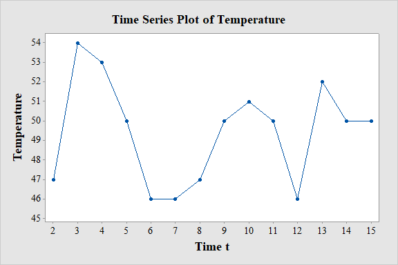
The obtained time series plot represents a cyclic pattern of temperature.
Explanation of Solution
Given info:
The data represents the observed value of response variable x at time t. The observed values are
Calculation:
Software Procedure:
Step-by-step procedure to draw the time series plot for temperature using the MINITAB software:
- Choose Graph > Time Series Plot.
- Choose Simple, and then click OK.
- In Series, enter the column of Temperature.
- Click OK.
Observation:
Time series plot shows that the highest temperature is at time 3 and the lowest temperature is at time 6 and 7. From the graph it can be concluded that temperature oscillates with the change in time. Overall the plot represents a cyclic pattern of temperature.
b.
Find the smoothed value
b.
Answer to Problem 82SE
Smoothed values
| Time t | ||
| 2 | 47 | 47 |
| 3 | 54 | 47.7 |
| 4 | 53 | 48.2 |
| 5 | 50 | 48.4 |
| 6 | 46 | 48.2 |
| 7 | 46 | 48 |
| 8 | 47 | 47.9 |
| 9 | 50 | 48.1 |
| 10 | 51 | 48.4 |
| 11 | 50 | 48.5 |
| 12 | 46 | 48.3 |
| 13 | 52 | 48.6 |
| 14 | 50 | 48.8 |
| 15 | 50 | 48.9 |
Smoothed values
| Time t | ||
| 2 | 47 | 47 |
| 3 | 54 | 50.5 |
| 4 | 53 | 51.8 |
| 5 | 50 | 50.9 |
| 6 | 46 | 48.4 |
| 7 | 46 | 47.2 |
| 8 | 47 | 47.1 |
| 9 | 50 | 48.6 |
| 10 | 51 | 49.8 |
| 11 | 50 | 49.9 |
| 12 | 46 | 47.9 |
| 13 | 52 | 50 |
| 14 | 50 | 50 |
| 15 | 50 | 50 |
Explanation of Solution
Calculation:
The exponential smoothing equation is
Smoothed values
Here, to calculate the smoothed value
That is,
Moreover, it is given that
Hence, the smoothed value
Thus, the smoothed value at time 2 is
The smoothed value
Thus, the smoothed value at time 3 is
Similarly, smoothed values for the remaining times are given below:
| Time t | ||
| 2 | 47 | 47 |
| 3 | 54 | 47.7 |
| 4 | 53 | 48.2 |
| 5 | 50 | 48.4 |
| 6 | 46 | 48.2 |
| 7 | 46 | 48 |
| 8 | 47 | 47.9 |
| 9 | 50 | 48.1 |
| 10 | 51 | 48.4 |
| 11 | 50 | 48.5 |
| 12 | 46 | 48.3 |
| 13 | 52 | 48.6 |
| 14 | 50 | 48.8 |
| 15 | 50 | 48.9 |
Smoothed values
Here, to calculate the smoothed value
That is,
Moreover, it is given that
Hence, the smoothed value
Thus, the smoothed value at time 2 is
The smoothed value
Thus, the smoothed value at time 3 is
Similarly, smoothed values for the remaining times are given below:
| Time t | ||
| 2 | 47 | 47 |
| 3 | 54 | 50.5 |
| 4 | 53 | 51.8 |
| 5 | 50 | 50.9 |
| 6 | 46 | 48.4 |
| 7 | 46 | 47.2 |
| 8 | 47 | 47.1 |
| 9 | 50 | 48.6 |
| 10 | 51 | 49.8 |
| 11 | 50 | 49.9 |
| 12 | 46 | 47.9 |
| 13 | 52 | 50 |
| 14 | 50 | 50 |
| 15 | 50 | 50 |
c.
Find the number of values of
Find the change in the coefficient of
c.
Answer to Problem 82SE
The value of
The coefficient on
Explanation of Solution
Calculation:
The exponential smoothing equation is
Substituting the value,
Substituting the value,
Continuing the same computational procedure till the value of
Now, the equation reduces as follows:
The value of
Now, the exponential smoothing equation
Here, from the above obtained equation it is seen that the value of
Here, form the equation it can be said that the coefficient of
Moreover, the smoothing constant
That is,
Hence the value of
Therefore, the coefficient on
c.
Explain the sensitivity of the initialization of
c.
Answer to Problem 82SE
The smoothed series
Explanation of Solution
Calculation:
From part (c), the exponential smoothing equation is,
The substitution of of
Here, form the equation it can be said that the coefficient of
Moreover, the smoothing constant
That is,
Hence the value of
Therefore, the smoothed series
Want to see more full solutions like this?
Chapter 1 Solutions
Probability and Statistics for Engineering and the Sciences


- 1. Consider the Gaussian distribution N (m, σ2).(a) Show that the pdf integrates to 1.(b) Show that the mean is m and the variance is σ.arrow_forwardIf X(t) is a continuous-time random process with mean value of m and variance of s^2, what is the value of the autocorrelation function at time lag tau=0?arrow_forwardA random variable ? is the output of an engineering process, and ? is uniformlydistributed. The PDF of ? is equal to 1/10 for any positive x smaller than or equal to 10, and it is 0otherwise. If you take a random sample of 30 observations, what is the approximate probabilitydistribution of ?̅ − 3? (You need to find the mean and variance of this quantity and state yourassumptions)arrow_forward
- A random variable X is normally distributed with a mean of 100 and a variance of 100, and a random vari- able Y is normally distributed with a mean of 200 and a variance of 400. The random variables have a corre- lation coefficient equal to 0.5. Find the mean and vari- ance of the random variable: W = 5X + 4Yarrow_forward1. Suppose that X1, Xn is an iid random sample from a distribution with pdf f(x; sigma) = 1/2 * (sigma) * e ^ (- |x| / sigma) - infinity0 0(a) Find the method of moments estimator (MME) of \sigma. Hint: See the example in lecture notes. (b) Find the maximum likelihood estimator (MLE) of \sigma. Hint: See the example in lecture notes. (c) Use central limit theorem to find the large - sample asymptotic distribution of the MLE in part (b). (d) Suppose 10 independent observations were taken from the given distribution: (0.5, 0.8, 2.2, 1.6, 2.0, 2.8, 1.5, 0.9, 2.5, 1.8). What is the numerical value of the MLE? What is the numerical value of the estimated standard deviation (standard error) of the MLE?arrow_forwardTwo populations are surveyed using simple random samples. A sample of size n1 is used for population I, which has a population standard deviation of σ 1, and a sample of size n2 = 2n1 is used for population II, which has a population standard deviation σ 2 = 2 σ 1. For which of the two samples would you expect the sample mean to be more accurate?arrow_forward
- Suppose a quality control expert examines iterms for defects in a series of independent fixates, each of a fixed duration, and suppose that defects are present. Let p be the probability that the defect or flaw is detected and 1-p the probability that a defect or flaw is not detected. Let the r.v. X = the number of defects detected in n fixations. a. What is the pmf of X? b. What is the expected value of X = E(X)? c. What is the moment generating function (mgf) for the r.v. X (Remember to state the interval of validity for t)? d. Use it to find the Variance of X.arrow_forwardA time series {yt} follows an MA(2) model: Yt = 2 + Ut +0.54t-1 + 0.4ut-2. Assume that ut is a white noise series with a mean of O and a variance of 2. Please calculate Var(yt) (i.e. the variance of) 2.96 1.41 2.82 O 1.98arrow_forward34) If a population exhibits a skew of -5.00 and an excess kurtosis of 5.00 which of the following is true? The population mean exceeds the median. The population variance exceeds the standard deviation. The population standard deviation exceeds the variance. The population median equals the mean. The population median exceeds the mean.arrow_forward
- a hypothesis test produces a t statistic of t=2.3. if the researcher is using a two tailed test with a=0.05 how large does the sample have to bw in order to reject the null hypothesis?arrow_forwardThe time for the first widget to be manufactured each morning is random between 1 and 3 seconds with a pdf of f(x)=1/162(x-3)^2(x+6) for 0 < x < 6What is the cumulative distribution function, F(x)? What is the probability of a widget being made earlier than 4 s?Answer to four decimal places What is the probability of a widget being made later than 1.3 s?Answer to four decimal placesarrow_forwardA continuous random variable X has the PDF fx(x)=kx2, 0 < ? < 1.a) What is the value of k ?b) Find the variance of Xc) What is the value of m so that P[X<=m] = 1/2 ?d) Find the PDF of the new random variable Y obtained from X through the lineartransformation Y=4X+1.arrow_forward
 Algebra & Trigonometry with Analytic GeometryAlgebraISBN:9781133382119Author:SwokowskiPublisher:Cengage
 Glencoe Algebra 1, Student Edition, 9780079039897...AlgebraISBN:9780079039897Author:CarterPublisher:McGraw Hill