Chapter 10.1, Problem 29E

a.

To determine

Perform a chi-square distribution to test the given null hypothesis at the level of significance of $\alpha =0.05$.

Answer to Problem 29E

There is not enough evidence to conclude that the die is fair.

Explanation of Solution

Calculation:

A gambler rolls a die 600 times to find whether the dice is fair or not. The observed frequencies of outcomes are given. Assumed that $p_1$, $p_2$,…, $p_6$ are the probabilities of the die comes up 1, the die comes up 2,…, the die comes up 6, respectively.

It is known that probability of each outcome of a fair die is $\frac{1}{6}$.

The hypotheses are:

Null Hypothesis:

$H_0:p_1=p_2=\mathrm{...}=p_6=\frac{1}{6}$.

That is, the die is fair.

Alternative Hypothesis:

$H_1:\text{Not all }{p}_i\text{'}\text{s}\text{are same as }{H}_0\text{for }i=1,\mathrm{...},6$.

That is, the die is not fair.

Expected frequencies:

The expected frequencies are defined as $E_1=n{p}_1$, $E_2=n{p}_2$ and so on, for the probabilities of $p_1$, $p_2$,… are specified by null hypothesis $H_0$ with the total number of trial n.

The total number of trial is obtained as,

$\begin{array}{c}n=113+101+106+81+108+91\\ =600\end{array}$.

Thus, the expected frequencies are,

Outcome	Expected frequencies $\left(E_i=n{p}_i,\text{ for all }i=1,2,\mathrm{...},6\right)$
1	$\left(600\right)\left(\frac{1}{6}\right)=100$
2	$\left(600\right)\left(\frac{1}{6}\right)=100$
3	$\left(600\right)\left(\frac{1}{6}\right)=100$
4	$\left(600\right)\left(\frac{1}{6}\right)=100$
5	$\left(600\right)\left(\frac{1}{6}\right)=100$
6	$\left(600\right)\left(\frac{1}{6}\right)=100$

The observed and expected frequencies are obtained as,

Outcome	Observed Frequencies	Expected frequencies
1	113	100
2	101	100
3	106	100
4	81	100
5	108	100
6	91	100

Chi-Square statistic:

The chi-square statistic is obtained as ${\chi }^2={\displaystyle \sum \frac{{\left(O-E\right)}^2}{E}}$ where $O_1,O_2,\mathrm{...},O_k$ be the observed frequencies and $E_1,E_2,\mathrm{...},E_k$ be the expected frequencies for k number of categories.

Now,

Outcome	Observed frequencies (O)	Expected frequencies (E)	${\left(O-E\right)}^2$	$\frac{{\left(O-E\right)}^2}{E}$
1	113	100	169	1.69
2	101	100	1	0.01
3	106	100	36	0.36
4	81	100	361	3.61
5	108	100	64	0.64
6	91	100	81	0.81
Total	600	600	712	7.12

Thus, the value of ${\chi }^2$ is 7.12.

Degrees of freedom:

It is known that under the null hypothesis $H_0$ the test statistic ${\chi }^2={\displaystyle \sum \frac{{\left(O-E\right)}^2}{E}}$ follows chi-square distribution with $k-1$ degrees of freedom for k number of categories, provided that all the expected frequencies are greater than or equal to 5.

In the given question there are 6 categories (Outcome). Thus, $k=6$.

Hence, the degrees of freedom is $6-1=5$.

Thus, the degree of freedom is 5.

Level of significance:

The level of significance is given as 0.05.

Critical value:

In a test of hypotheses the critical value is the point by which one can reject or accept the null hypothesis.

Software procedure:

Step-by-step software procedure to obtain critical value using MINITAB software is as follows:

• Select Graph > Probability distribution plot > view probability
• Select Chi -Square under distribution.
• In Degrees of freedom, enter 5.
• Choose Probability Value and Right Tail for the region of the curve to shade.
• Enter the Probability value as 0.05 under shaded area.
• Select OK.
• Output using MINITAB software is given below:

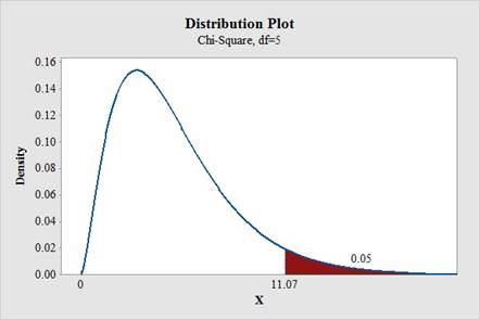
Hence, the critical value at $\alpha =0.05$ is 11.07.

  Rejection rule:

If the ${\chi }^2$ value is greater than or equal to critical value, that is ${\chi }^2\ge {\chi }_{\alpha ;k-1}^2$, then reject the null hypothesis $H_0$. Otherwise, do not reject $H_0$.

Conclusion:

Here, the ${\chi }^2$ value is less than the critical value.

That is, ${\chi }^2\left(=7.12\right)<{\chi }_{0.05,5}^2\left(=11.07\right)$

Thus, the decision is “fail to reject the null hypothesis”.

Thus, there is not enough evidence to conclude that the die is fair.

b.

To determine

Find the P-values for each of these tests.

Explanation of Solution

The P-values for outcome 1, outcome 2, outcome 3, outcome 4, outcome 5 and outcome 5 are 0.16728, 0.9298, 0.5106, 0.03662, 0.3804 and 0.3236, respectively.

Calculation:

The null hypothesis is given as $H_0:p_i=\frac{1}{6},\text{for each }{p}_i$.

It is known that probability of each outcome of a fair die is $\frac{1}{6}$.

Assume that p is the population proportion of individuals for specified category.

Thus, in the given problem $p_i=\frac{1}{6}$ for all $i=1,2,\mathrm{...},6$.

It is also assumed that $p_0$ and $\widehat{p}$ are the population proportion specified by $H_0$ and the sample proportion of individuals for in specified category, respectively.

The sample proportion $\widehat{p}$ can be defined as $\widehat{p}=\frac{x}{n}$ where x is the number of individuals in the sample in the specified category and n is the sample size.

The assumptions for performing a Hypothesis Test for a population proportion are defined as,

• The sample is simple random sample.
• The population size is at least 20 times of the sample size.
• The individuals in the population are divided into two categories.
• The minimum values of both $n{p}_0$ and $n\left(1-p_0\right)$ are 10.

The gambler rolls the die 600 times and all the outcomes in the population have the equal probability of being included in the sample. Hence, the given sample is a simple random sample.

The gambler can throw the dice infinitely many times. Hence, population size is more than 20 times of the sample size

The outcomes can be classified in two categories. One is occurring of a particular face and another is not occurring of that particular face.

The value of n and $p_0$ are 600 and $\frac{1}{6}$, respectively.

Hence,

$\begin{array}{c}n{p}_0=\left(600\right)\left(\frac{1}{6}\right)\\ =100\\ \ge 10\end{array}$

And,

$\begin{array}{c}n\left(1-p_0\right)=\left(600\right)\left(1-\frac{1}{6}\right)\\ =\left(600\right)\left(\frac{5}{6}\right)\\ =500\\ \ge 10\end{array}$

Now, as all the assumptions of for performing a Hypothesis Test for a population proportion are satisfied, then one can proceed to perform a Hypothesis Test for a population proportion.

For outcome 1:

The hypotheses are:

Null Hypothesis:

$H_0:p_1=\frac{1}{6}$.

That is, the probability of occurring one in a fair die is $\frac{1}{6}$.

Alternate Hypothesis:

$H_1:p_1\ne \frac{1}{6}$.

That is, the probability of occurring one in a fair die is not equal to $\frac{1}{6}$.

Level of significance:

The level of significance is given as 0.05.

The test statistic z is defend as $z=\frac{\widehat{p}-p_0}{\sqrt{\frac{p_0\left(1-p_0\right)}{n}}}$.

It is already found that $p_0=\frac{1}{6}$.

Now, the number of individuals in the sample for the outcome 1 is 113 and the sample size is 600.

Hence,

$\begin{array}{c}\widehat{p}=\frac{113}{600}\\ =0.188\end{array}$

Thus, the test statistic value is,

 $\begin{array}{c}z=\frac{\widehat{p}-p_0}{\sqrt{\frac{p_0\left(1-p_0\right)}{n}}}\\ =\frac{0.188-\frac{1}{6}}{\sqrt{\frac{\frac{1}{6}\left(1-\frac{1}{6}\right)}{600}}}\\ =\frac{0.021}{\sqrt{\frac{\frac{5}{36}}{600}}}\\ =\frac{0.021}{\sqrt{\frac{0.138}{600}}}\end{array}$

    $\begin{array}{c}=\frac{0.021}{\sqrt{0.00023}}\\ =\frac{0.021}{0.0152}\\ =1.381\end{array}$

P-value:

Software procedure:

Step-by-step software procedure to obtain P-value using MINITAB software is as follows:

• Select Graph > Probability distribution plot > view probability
• Select Norma under distribution.
• Enter Mean as 0 and enter Standard deviation as 1.
• Choose X Value and Both Tail for the region of the curve to shade.
• Enter the X value as 1.381 under shaded area.
• Select OK.
• Output using MINITAB software is given below:

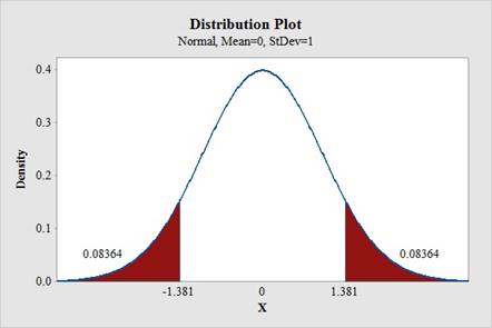
Hence, the P-value is  $2\times 0.08364=\underset{\_}{0.16728}.$

For outcome 2:

The hypotheses are:

Null Hypothesis:

$H_0:p_2=\frac{1}{6}$.

That is, the probability of occurring two in a fair die is $\frac{1}{6}$.

Alternate Hypothesis:

$H_1:p_2\ne \frac{1}{6}$.

That is, the probability of occurring two in a fair die is not equal to $\frac{1}{6}$.

Level of significance:

The level of significance is given as 0.05.

The test statistic z is defend as $z=\frac{\widehat{p}-p_0}{\sqrt{\frac{p_0\left(1-p_0\right)}{n}}}$.

It is already found that $p_0=\frac{1}{6}$.

Now, the number of individuals in the sample for the outcome 2 is 2.2 and the sample size is 600.

Hence,

$\begin{array}{c}\widehat{p}=\frac{101}{600}\\ =0.168\end{array}$

Thus, the test statistic value is,

 $\begin{array}{c}z=\frac{\widehat{p}-p_0}{\sqrt{\frac{p_0\left(1-p_0\right)}{n}}}\\ =\frac{0.168-\frac{1}{6}}{\sqrt{\frac{\frac{1}{6}\left(1-\frac{1}{6}\right)}{600}}}\\ =\frac{0.0013}{\sqrt{\frac{\frac{5}{36}}{600}}}\\ =\frac{0.0013}{\sqrt{\frac{0.138}{600}}}\end{array}$

    $\begin{array}{c}=\frac{0.0013}{\sqrt{0.00023}}\\ =\frac{0.0013}{0.0152}\\ \approx 0.088\end{array}$

P-value:

Software procedure:

Step-by-step software procedure to obtain P-value using MINITAB software is as follows:

• Select Graph > Probability distribution plot > view probability
• Select Norma under distribution.
• Enter Mean as 0 and enter Standard deviation as 1.
• Choose X Value and Both Tail for the region of the curve to shade.
• Enter the X value as 0.088 under shaded area.
• Select OK.
• Output using MINITAB software is given below:

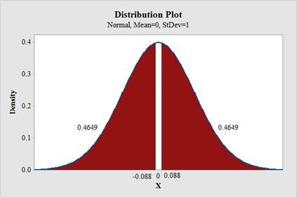
Hence, the P-value is  $2\times 0.4649=\underset{\_}{0.9298}$.

For outcome 3:

The hypotheses are:

Null Hypothesis:

$H_0:p_3=\frac{1}{6}$.

That is, the probability of occurring three in a fair die is $\frac{1}{6}$.

Alternate Hypothesis:

$H_1:p_3\ne \frac{1}{6}$.

That is, the probability of occurring three in a fair die is not equal to $\frac{1}{6}$.

Level of significance:

The level of significance is given as 0.05.

The test statistic z is defend as $z=\frac{\widehat{p}-p_0}{\sqrt{\frac{p_0\left(1-p_0\right)}{n}}}$.

It is already found that $p_0=\frac{1}{6}$.

Now, the number of individuals in the sample for the outcome 3 is 106 and the sample size is 600.

Hence,

$\begin{array}{c}\widehat{p}=\frac{106}{600}\\ \approx 0.177\end{array}$

Thus, the test statistic value is,

 $\begin{array}{c}z=\frac{\widehat{p}-p_0}{\sqrt{\frac{p_0\left(1-p_0\right)}{n}}}\\ =\frac{0.177-\frac{1}{6}}{\sqrt{\frac{\frac{1}{6}\left(1-\frac{1}{6}\right)}{600}}}\\ =\frac{0.01}{\sqrt{\frac{\frac{5}{36}}{600}}}\\ =\frac{0.01}{\sqrt{\frac{0.138}{600}}}\end{array}$

    $\begin{array}{c}=\frac{0.01}{\sqrt{0.00023}}\\ =\frac{0.01}{0.0152}\\ \approx 0.658\end{array}$

P-value:

Software procedure:

Step-by-step software procedure to obtain P-value using MINITAB software is as follows:

• Select Graph > Probability distribution plot > view probability
• Select Norma under distribution.
• Enter Mean as 0 and enter Standard deviation as 1.
• Choose X Value and Both Tail for the region of the curve to shade.
• Enter the X value as 0.658 under shaded area.
• Select OK.
• Output using MINITAB software is given below:

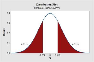
Hence, the P-value is  $2\times 0.2553=\underset{\_}{0.5106}.$ .

For outcome 4:

The hypotheses are:

Null Hypothesis:

$H_0:p_4=\frac{1}{6}$.

That is, the probability of occurring four in a fair die is $\frac{1}{6}$.

Alternate Hypothesis:

$H_1:p_4\ne \frac{1}{6}$.

That is, the probability of occurring four in a fair die is not equal to $\frac{1}{6}$.

Level of significance:

The level of significance is given as 0.05.

The test statistic z is defend as $z=\frac{\widehat{p}-p_0}{\sqrt{\frac{p_0\left(1-p_0\right)}{n}}}$.

It is already found that $p_0=\frac{1}{6}$.

Now, the number of individuals in the sample for the outcome 4 is 81 and the sample size is 600.

Hence,

$\begin{array}{c}\widehat{p}=\frac{81}{600}\\ =0.135\end{array}$

Thus, the test statistic value is,

 $\begin{array}{c}z=\frac{\widehat{p}-p_0}{\sqrt{\frac{p_0\left(1-p_0\right)}{n}}}\\ =\frac{0.135-\frac{1}{6}}{\sqrt{\frac{\frac{1}{6}\left(1-\frac{1}{6}\right)}{600}}}\\ =\frac{-0.0317}{\sqrt{\frac{\frac{5}{36}}{600}}}\\ =\frac{-0.0317}{\sqrt{\frac{0.138}{600}}}\end{array}$

    $\begin{array}{c}=\frac{-0.0317}{\sqrt{0.00023}}\\ =\frac{-0.0317}{0.0152}\\ =-2.09\end{array}$

Level of significance:

The level of significance is given as 0.05.

P-value:

Software procedure:

Step-by-step software procedure to obtain P-value using MINITAB software is as follows:

• Select Graph > Probability distribution plot > view probability
• Select Norma under distribution.
• Enter Mean as 0 and enter Standard deviation as 1.
• Choose X Value and Both Tail for the region of the curve to shade.
• Enter the X value as –2.09 under shaded area.
• Select OK.
• Output using MINITAB software is given below:

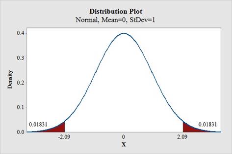
Hence, the P-value is  $2\times 0.01831=\underset{\_}{0.03662}.$ .

For outcome 5:

The hypotheses are:

Null Hypothesis:

$H_0:p_5=\frac{1}{6}$.

That is, the probability of occurring five in a fair die is $\frac{1}{6}$.

Alternate Hypothesis:

$H_1:p_5\ne \frac{1}{6}$.

That is, the probability of occurring five in a fair die is not equal to $\frac{1}{6}$.

Level of significance:

The level of significance is given as 0.05.

The test statistic z is defend as $z=\frac{\widehat{p}-p_0}{\sqrt{\frac{p_0\left(1-p_0\right)}{n}}}$.

It is already found that $p_0=\frac{1}{6}$.

Now, the number of individuals in the sample for the outcome 5 is 108 and the sample size is 600.

Hence,

$\begin{array}{c}\widehat{p}=\frac{108}{600}\\ =0.18\end{array}$

Thus, the test statistic value is,

 $\begin{array}{c}z=\frac{\widehat{p}-p_0}{\sqrt{\frac{p_0\left(1-p_0\right)}{n}}}\\ =\frac{0.18-\frac{1}{6}}{\sqrt{\frac{\frac{1}{6}\left(1-\frac{1}{6}\right)}{600}}}\\ =\frac{0.013}{\sqrt{\frac{\frac{5}{36}}{600}}}\\ =\frac{0.013}{\sqrt{\frac{0.138}{600}}}\end{array}$

    $\begin{array}{c}=\frac{0.013}{\sqrt{0.00023}}\\ =\frac{0.013}{0.0152}\\ =0.877\end{array}$

P-value:

Software procedure:

Step-by-step software procedure to obtain P-value using MINITAB software is as follows:

• Select Graph > Probability distribution plot > view probability
• Select Norma under distribution.
• Enter Mean as 0 and enter Standard deviation as 1.
• Choose X Value and Both Tail for the region of the curve to shade.
• Enter the X value as 0.877 under shaded area.
• Select OK.
• Output using MINITAB software is given below:

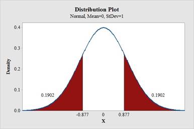
Hence, the P-value is  $2\times 0.1902=\underset{\_}{0.3804}$.

For outcome 6:

The hypotheses are:

Null Hypothesis:

$H_0:p_6=\frac{1}{6}$.

That is, the probability of occurring six in a fair die is $\frac{1}{6}$.

Alternate Hypothesis:

$H_1:p_6\ne \frac{1}{6}$.

That is, the probability of occurring six in a fair die is not equal to $\frac{1}{6}$.

Level of significance:

The level of significance is given as 0.05.

The test statistic z is defend as $z=\frac{\widehat{p}-p_0}{\sqrt{\frac{p_0\left(1-p_0\right)}{n}}}$.

It is already found that $p_0=\frac{1}{6}$.

Now, the number of individuals in the sample for the outcome 6 is 91 and the sample size is 600.

Hence,

$\begin{array}{c}\widehat{p}=\frac{91}{600}\\ =0.152\end{array}$

Thus, the test statistic value is,

 $\begin{array}{c}z=\frac{\widehat{p}-p_0}{\sqrt{\frac{p_0\left(1-p_0\right)}{n}}}\\ =\frac{0.152-\frac{1}{6}}{\sqrt{\frac{\frac{1}{6}\left(1-\frac{1}{6}\right)}{600}}}\\ =\frac{-0.015}{\sqrt{\frac{\frac{5}{36}}{600}}}\\ =\frac{-0.015}{\sqrt{\frac{0.138}{600}}}\end{array}$

    $\begin{array}{c}=\frac{-0.015}{\sqrt{0.00023}}\\ =\frac{-0.015}{0.0152}\\ \approx -0.987\end{array}$

P-value:

Software procedure:

Step-by-step software procedure to obtain P-value using MINITAB software is as follows:

• Select Graph > Probability distribution plot > view probability
• Select Norma under distribution.
• Enter Mean as 0 and enter Standard deviation as 1.
• Choose X Value and Both Tail for the region of the curve to shade.
• Enter the X value as –0.987 under shaded area.
• Select OK.
• Output using MINITAB software is given below:

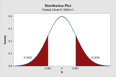
Hence, the P-value is  $2\times 0.1618=\underset{\_}{0.3236}$.

c.

To determine

Prove that the hypothesis $H_0:p_4=\frac{1}{6}$ is rejected at the level of significance of $\alpha =0.05$.

Explanation of Solution

Calculation:

It is known that probability of each outcome of a fair die is $\frac{1}{6}$.

Assume that p is the population proportion of individuals for specified category.

Thus, in the given problem $p_i=\frac{1}{6}$ for all $i=1,2,\mathrm{...},6$.

It is also assumed that $p_0$ and $\widehat{p}$ are the population proportion specified by $H_0$ and the sample proportion of individuals for in specified category, respectively.

The sample proportion $\widehat{p}$ can be defined as $\widehat{p}=\frac{x}{n}$ where x is the number of individuals in the sample in the specified category and n is the sample size.

The assumptions for performing a Hypothesis Test for a population proportion are defined as,

• The sample is simple random sample.
• The population size is at least 20 times of the sample size.
• The individuals in the population are divided into two categories.
• The minimum values of both $n{p}_0$ and $n\left(1-p_0\right)$ are 10.

The gambler rolls the die 600 times and all the outcomes in the population have the equal probability of being included in the sample. Hence, the given sample is a simple random sample.

The gambler can throw the dice infinitely many times. Hence, population size is more than 20 times of the sample size

The outcomes can be classified in two categories. One is occurring of a particular face and another is not occurring of that particular face.

The value of n and $p_0$ are 600 and $\frac{1}{6}$, respectively.

Hence,

$\begin{array}{c}n{p}_0=\left(600\right)\left(\frac{1}{6}\right)\\ =100\\ \ge 10\end{array}$

And,

$\begin{array}{c}n\left(1-p_0\right)=\left(600\right)\left(1-\frac{1}{6}\right)\\ =\left(600\right)\left(\frac{5}{6}\right)\\ =500\\ \ge 10\end{array}$

Now, as all the assumptions of for performing a Hypothesis Test for a population proportion are satisfied, then one can proceed to perform a Hypothesis Test for a population proportion.

Step 1:

The hypotheses are:

Null Hypothesis:

$H_0:p_4=\frac{1}{6}$.

That is, the probability of occurring four in a fair die is $\frac{1}{6}$.

Alternative Hypothesis:

$H_1:p_4\ne \frac{1}{6}$.

That is, the probability of occurring four in a fair die is not equal to $\frac{1}{6}$.

Step 2:

Level of significance:

The level of significance is given as 0.05.

Step 3:

The test statistic z is defend as $z=\frac{\widehat{p}-p_0}{\sqrt{\frac{p_0\left(1-p_0\right)}{n}}}$.

It is already found that $p_0=\frac{1}{6}$.

Now, the number of individuals in the sample for the outcome 4 is 81 and the sample size is 600.

Hence,

$\begin{array}{c}\widehat{p}=\frac{81}{600}\\ =0.135\end{array}$

Thus, the test statistic value is,

 $\begin{array}{c}z=\frac{\widehat{p}-p_0}{\sqrt{\frac{p_0\left(1-p_0\right)}{n}}}\\ =\frac{0.135-\frac{1}{6}}{\sqrt{\frac{\frac{1}{6}\left(1-\frac{1}{6}\right)}{600}}}\\ =\frac{-0.0317}{\sqrt{\frac{\frac{5}{36}}{600}}}\\ =\frac{-0.0317}{\sqrt{\frac{0.138}{600}}}\end{array}$

    $\begin{array}{c}=\frac{-0.0317}{\sqrt{0.00023}}\\ =\frac{-0.0317}{0.0152}\\ =-2.09\end{array}$

Step 4:

Level of significance:

The level of significance is given as 0.05.

P-value:

Software procedure:

Step-by-step software procedure to obtain P-value using MINITAB software is as follows:

• Select Graph > Probability distribution plot > view probability
• Select Norma under distribution.
• Enter Mean as 0 and enter Standard deviation as 1.
• Choose X Value and Both Tail for the region of the curve to shade.
• Enter the X value as –2.09 under shaded area.
• Select OK.
• Output using MINITAB software is given below:

Hence, the P-value is $2\times 0.01831=0.03662$ .

  Rejection rule:

Decision based on the P-value method:

• If $P\text{- value}\le \alpha$, reject $H_0$.
• If $P\text{-}\text{value}>\alpha$, fail to reject $H_0$.

Step 5:

The significance level is, $\alpha =0.05$ and the P-value is 0.03662.

Here, the P-value of 0.03662 is less than the significance level 0.05.

That is, $P\text{-value}\left(=0.03662\right)<\alpha \left(=0.05\right)$.

Step 6:

Conclusion:

Therefore, there is no evidence to suggest that probability of occurring four in a fair die is $\frac{1}{6}$.

Hence, it is proved that the hypothesis $H_0:p_4=\frac{1}{6}$ is rejected at the level of significance of $\alpha =0.05$.