Understanding Basic Statistics
8th Edition
ISBN: 9781337558075
Author: Charles Henry Brase, Corrinne Pellillo Brase
Publisher: Cengage Learning
bartleby

Concept explainers

bartleby

Videos

Question
Book Icon
Chapter 10.2, Problem 22P
To determine

The verification of x¯14.00,s12.38,x¯25.5,s22.78 using calculator.

Expert Solution
Check Mark

Explanation of Solution

To find the required statistics using the Minitab, follow the below instructions:

Step 1: Go to the Minitab software.

Step 2: Go to Stat > Basic statistics > Display Descriptive statistics.

Step 3: Select dataset ‘Field A’ and dataset ‘Field B’ in variables.

Step 4: Click on OK.

The obtained output is:

Statistics

Variable N N* Mean SE Mean StDev Minimum Q1 Median Q3 Maximum
Sample 1 7 0 4.000 0.900 2.380 2.000 2.000 3.000 6.000 8.000
Sample 2 8 0 5.500 0.982 2.777 2.000 3.000 5.500 7.750 10.000

From the above output we have find that the values of x¯1,s1,x¯2,s2 are approximately x¯14.00,s12.38,x¯25.5,s22.78.

(a)

(i)

To determine

The level of significance, null hypothesis and alternate hypothesis.

(a)

(i)

Expert Solution
Check Mark

Answer to Problem 22P

Solution: The hypotheses are H0:μ1=μ2andH1:μ1<μ2. The level of significance is 0.05.

Explanation of Solution

The level of significance is 0.05.Since, we want to conduct a test of the claim that population mean time lost due to stressors is greater than the population mean time lost due to intimidators. Therefore the null hypothesis is H0:μ1=μ2 v/s alternative hypothesisis H1:μ1<μ2.

(ii)

To determine

To find: The sampling distribution that should be used along with assumptions and compute the value of the sample test statistic.

(ii)

Expert Solution
Check Mark

Answer to Problem 22P

Solution: We can use student’s t distribution. The sample test statisticis t=1.13.

Explanation of Solution

Calculation:

Let’s assume that the population distributions of time lost due to intimidators and time lost due to stressors are each mound shape and approximately symmetrical. The population standard deviation (σ1andσ2) are also unknown, so we can assume that sample test statistics follows a Student’s t-distribution.

Using x¯1=4.00,x¯2=5.5,μ1-μ2=0,s12=(2.38)2,s22=(2.78)2,n1=7,n2=8 where x¯1 and x¯2 are the sample means for first sample and second sample respectively.

s12 and s22 are the sample variance for first sample and second sample respectively.

n1 and n2 are the sample size for first sample and second sample respectively.

The sample test statistic t is calculated as follows:

t=(x¯1-x¯2)-(μ1-μ2)s12n1+s22n2t=(4.005.50)0(2.38)27+(2.78)28t=1.1258t1.13

Thus the test statistic is t=1.13.

(iii)

To determine

To find: The P-value of the test statistic and sketch the sampling distribution showing the area corresponding to the P-value.

(iii)

Expert Solution
Check Mark

Answer to Problem 22P

Solution: The P-value of the sample test statistic is 0.1508.

Explanation of Solution

Calculation:

The given hypothesis test is two tailed.

Pvalue =P(t<1.13)

D.F = Smaller of n11 and n21.

D.F=n11D.F=71D.F=6

By using table 4 from Appendix

0.125<pvalue<0.250

Graph:

To draw the required graphs using the Minitab, follow the below instructions:

Step 1: Go to the Minitab software.

Step 2: Go to Graph > Probability distribution plot > View probability.

Step 3: Select ‘t’ and enter D.f = 6.

Step 4: Click on the Shaded area > X value.

Step 5: Enter X-value as -1.13 and select ‘Left tail’.

Step 6: Click on OK.

The obtained distribution graph is:
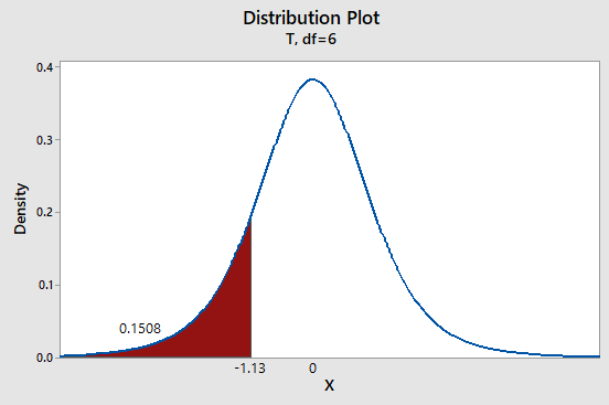
Understanding Basic Statistics, Chapter 10.2, Problem 22P

P-value = 0.1508

(iv)

To determine

Whether we reject or fail to reject the null hypothesis and whether the data is statistically significant for a level of significance of 0.05.

(iv)

Expert Solution
Check Mark

Answer to Problem 22P

Solution: The P-value >α, hence we fail to reject H0. The data is not statistically significant for a level of significance of 0.05.

Explanation of Solution

The P-value (0.1508) is greater than the level of significance (α) of 0.05. Therefore we don’t have enough evidence to reject the null hypothesis H0 i.e. the P-value is not statistically significant.

(v)

To determine

The interpretation for the conclusion.

(v)

Expert Solution
Check Mark

Answer to Problem 22P

Solution: There is not enough evidence to conclude that population mean time lost due to stressors is greater than the population mean time lost due to intimidators.

Explanation of Solution

The P-value (0.1508) is greater than the level of significance (α) of 0.05. Therefore we don’t have enough evidence to reject the null hypothesis H0 i.e. the P-value is not statistically significant. There is not enough evidence to conclude that population mean time lost due to stressors is greater than the population mean time lost due to intimidators.

(b)

To determine

To find: The 90%confidence interval for μ1-μ2 and explain the meaning of the confidence interval in the context of the problem.

(b)

Expert Solution
Check Mark

Answer to Problem 22P

Solution:

The 90% confidence interval for the difference of two means is 4.09<(μ1μ2)<1.09.

Explanation of Solution

Calculation:

The critical t-value for a two-tailed area of 0.10 is 1.943.

The difference of two means is

(x¯1 - x¯2)=4.005.50(x¯1 - x¯2)=1.50

Now, the margin of error is computed as follows:

E=tcs12n1+s22n2E=1.943(2.38)27+(2.78)28E=2.5888E2.59

Now the confidence interval for the difference of two means;

(x¯1x¯2)E<(μ1μ2)<(x¯1x¯2)+E1.502.59<(μ1μ2)<1.50+2.594.09<(μ1μ2)<1.09

The confidence interval for the difference of two means is 4.09<(μ1μ2)<1.09.

Interpretation:

At the 90% confidence level, we see that the difference of means ranges from negative to positives values. We cannot tell from this interval if population mean time lost due to stressors is greater than the population mean time lost due to intimidators.

Want to see more full solutions like this?

Subscribe now to access step-by-step solutions to millions of textbook problems written by subject matter experts!

Chapter 10 Solutions

Understanding Basic Statistics

Ch. 10.1 - For Problems 9-17 assume that the distribution of...Ch. 10.1 - For Problems 9-17 assume that the distribution of...Ch. 10.1 - For Problems 9-17 assume that the distribution of...Ch. 10.1 - Prob. 14PCh. 10.1 - For Problems 9-17 assume that the distribution of...Ch. 10.1 - For Problems 9-17 assume that the distribution of...Ch. 10.1 - Prob. 17PCh. 10.1 - Expand Your Knowledge: Confidence Intervals for d...Ch. 10.1 - Prob. 19PCh. 10.1 - Prob. 20PCh. 10.2 - Statistical Literacy Consider a hypothesis test of...Ch. 10.2 - Prob. 2PCh. 10.2 - Prob. 3PCh. 10.2 - Prob. 4PCh. 10.2 - Critical Thinking Josh and Kendra each calculated...Ch. 10.2 - Critical Thinking If a 90% confidence interval for...Ch. 10.2 - Basic Computation: Paired Differences Test For a...Ch. 10.2 - Basic Computation: Texting 12 Two populations have...Ch. 10.2 - Basic Computation: Testing- 12 A random sample of...Ch. 10.2 - Basic Computation: Testing 12 Two populations have...Ch. 10.2 - Please provide the following information for...Ch. 10.2 - Please provide the following information for...Ch. 10.2 - Please provide the following information for...Ch. 10.2 - Please provide the following information for...Ch. 10.2 - Please provide the following information for...Ch. 10.2 - Please provide the following information for...Ch. 10.2 - Please provide the following information for...Ch. 10.2 - Please provide the following information for...Ch. 10.2 - Please provide the following information for...Ch. 10.2 - Please provide the following information for...Ch. 10.2 - Prob. 21PCh. 10.2 - Prob. 22PCh. 10.2 - Prob. 23PCh. 10.2 - Prob. 24PCh. 10.2 - Prob. 25PCh. 10.2 - Critical Region Method: Testing 12;1,2Known Redo...Ch. 10.3 - Statistical Literacy Consider a hypothesis test of...Ch. 10.3 - Statistical Literacy Consider a hypothesis test of...Ch. 10.3 - Critical Thinking Consider two independent...Ch. 10.3 - Critical Thinking If a 90% confidence interval for...Ch. 10.3 - Prob. 5PCh. 10.3 - Basic Computation: Testing p1p2 For one binomial...Ch. 10.3 - Federal Tax Money: Art Funding Would you favor...Ch. 10.3 - Art Funding: Politics Would you favor spending...Ch. 10.3 - Sociology: Trusting People Generally speaking,...Ch. 10.3 - Political Science: Voters This problem is based on...Ch. 10.3 - Extraterrestrials: Believe It? Based on...Ch. 10.3 - Art: Polities Do you prefer paintings in which the...Ch. 10.3 - Prob. 13PCh. 10.3 - Critical Region Method: Testing p1p2 Redo Problem...Ch. 10.3 - Basic Computation: Confidence Inters al for p1p2...Ch. 10.3 - Prob. 16PCh. 10.3 - Myers-Briggs: Marriage Counseling Isabel Myers was...Ch. 10.3 - Myers-Briggs: Marriage Counseling Most married...Ch. 10.3 - Navajo Culture: Traditional Hogans S. C. Jett is a...Ch. 10.3 - Archaeology: Cultural Affiliation "Unknown...Ch. 10.3 - Critical Thinking: Different Confidence Levels (a)...Ch. 10.3 - Focus Problem: Wood Duck Nests In the Focus...Ch. 10 - Statistical Literacy and Terminology When are two...Ch. 10 - 2. Statistical Literacy and Terminology When are...Ch. 10 - For each hypothesis test in Problems 3-10, please...Ch. 10 - For each hypothesis test in Problems 3-10, please...Ch. 10 - For each hypothesis test in Problems 3-10, please...Ch. 10 - For each hypothesis test in Problems 3-10, please...Ch. 10 - For each hypothesis test in Problems 3-10, please...Ch. 10 - Prob. 8CRCh. 10 - For each hypothesis test in Problems 3-10, please...Ch. 10 - For each hypothesis test in Problems 3-10, please...Ch. 10 - Prob. DHGPCh. 10 - In there a relationship between confidence...
Knowledge Booster
Background pattern image
Statistics
Learn more about
Need a deep-dive on the concept behind this application? Look no further. Learn more about this topic, statistics and related others by exploring similar questions and additional content below.
Recommended textbooks for you
Text book image
MATLAB: An Introduction with Applications
Statistics
ISBN:9781119256830
Author:Amos Gilat
Publisher:John Wiley & Sons Inc
Text book image
Probability and Statistics for Engineering and th...
Statistics
ISBN:9781305251809
Author:Jay L. Devore
Publisher:Cengage Learning
Text book image
Statistics for The Behavioral Sciences (MindTap C...
Statistics
ISBN:9781305504912
Author:Frederick J Gravetter, Larry B. Wallnau
Publisher:Cengage Learning
Text book image
Elementary Statistics: Picturing the World (7th E...
Statistics
ISBN:9780134683416
Author:Ron Larson, Betsy Farber
Publisher:PEARSON
Text book image
The Basic Practice of Statistics
Statistics
ISBN:9781319042578
Author:David S. Moore, William I. Notz, Michael A. Fligner
Publisher:W. H. Freeman
Text book image
Introduction to the Practice of Statistics
Statistics
ISBN:9781319013387
Author:David S. Moore, George P. McCabe, Bruce A. Craig
Publisher:W. H. Freeman
The Shape of Data: Distributions: Crash Course Statistics #7; Author: CrashCourse;https://www.youtube.com/watch?v=bPFNxD3Yg6U;License: Standard YouTube License, CC-BY
Shape, Center, and Spread - Module 20.2 (Part 1); Author: Mrmathblog;https://www.youtube.com/watch?v=COaid7O_Gag;License: Standard YouTube License, CC-BY
Shape, Center and Spread; Author: Emily Murdock;https://www.youtube.com/watch?v=_YyW0DSCzpM;License: Standard Youtube License