
Concept explainers
Videos
For Exercises 28 through 33, do a complete
a. Draw a
b. Compute the
c. State the hypotheses.
d. Test the hypotheses at α = 0.05. Use Table I.
e. Determine the regression line equation if r is significant.
f. Plot the regression line on the scatter plot, if appropriate.
g. Summarize the results.
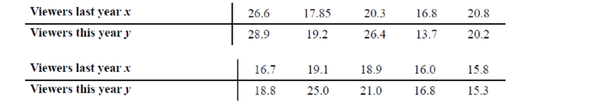
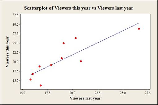
32. Television Viewers A television executive selects 10 television shows and compares the average number of viewers the show had last year with the average number of viewers this year. The data (in millions) are shown. Describe the relationship.
a.
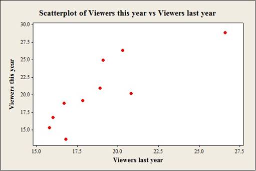
To construct: The scatterplot for the variablesthe average number of viewers the show hadlast year and the average number of viewers this year.
Answer to Problem 32E
Output using the MINITAB software is given below:
Explanation of Solution
Given info:
The data shows the average number of viewers the show hadlast year (x) and the average number of viewers this year(y) values.
Calculation:
Step by step procedure to obtain scatterplot using the MINITAB software:
- Choose Graph > Scatterplot.
- Choose Simple and then click OK.
- Under Y variables, enter a column ofViewers last year.
- Under X variables, enter a column of Viewers this year.
- Click OK.
b.
To compute: The value of the correlation coefficient.
Answer to Problem 32E
The value of the correlation coefficientis 0.839.
Explanation of Solution
Calculation:
Correlation coefficient r:
Software Procedure:
Step-by-step procedure to obtain the ‘correlation coefficient’ using the MINITAB software:
- Select Stat >Basic Statistics > Correlation.
- In Variables, select x and y from the box on the left.
- Click OK.
Output using the MINITAB software is given below:
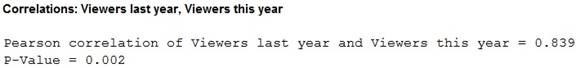
From the MINITAB output, the value of the correlation is 0.839.
c.
To state: The hypothesis.
Answer to Problem 32E
The null hypothesis is
The alternative hypothesis is
Explanation of Solution
Calculation:
The hypotheses are given below:
Null hypothesis:
That is, there is no linear relation betweenthe average number of viewers the show hadlast year and the average number of viewers this year.
Alternative hypothesis:
That is, there is a linear relationbetween the average number of viewers the show hadlast year and the average number of viewers this year.
d.
To test: The significance of the correlation coefficient at
Answer to Problem 32E
The conclusion is that, there is a sufficient evidence to support the claim that linear relation betweenthe average number of viewers the show had last year and the average number of viewers this year.
Explanation of Solution
Given info:
The level of significance is
Calculation:
The sample size is 10.
The formula to find the degrees of the freedom is
That is,
From the “TABLE –I: Critical Values for the PPMC”, the critical value for 4 degrees of freedom and
Rejection Rule:
If the absolute value of r is greater than the critical value then reject the null hypothesis.
Conclusion:
From part (b), the value of r is0.839 that is the absolute value of r is 0.839.
Here, the absolute value of r is greater than the critical value
That is,
By the rejection rule,reject the null hypothesis.
There is sufficient evidence to support the claim that “there is alinear relation betweenthe average number of viewers the show had last year and the average number of viewers this year”.
e.
To find: The regression equation for the given data.
Answer to Problem 32E
The regression equation for the given datais
Explanation of Solution
Calculation:
Regression:
Software procedure:
Step by step procedure to obtain the regression equation using the MINITAB software:
- Choose Stat > Regression > Regression.
- In Responses, enter the column ofViewers this year.
- In Predictors, enter the column ofViewers last year.
- Click OK.
Output using the MINITAB software is given below:
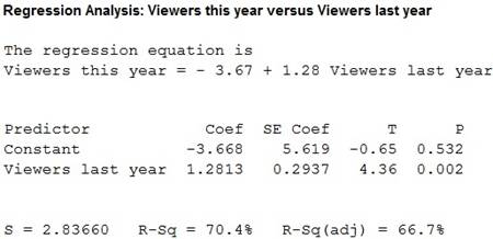
Thus, regression equation for the given datais
f.
To construct: The scatterplot for the variablesthe average number of viewers the show hadlast year and the average number of viewers this year.
Answer to Problem 32E
Output using the MINITAB software is given below:
Explanation of Solution
Calculation:
Step by step procedure to obtain scatterplot using the MINITAB software:
- Choose Graph > Scatterplot.
- Choose with line and then click OK.
- Under Y variables, enter a column of Viewers last year.
- Under X variables, enter a column of Viewers this year.
- Click OK.
g.
To summarize: The results.
Answer to Problem 32E
Explanation of Solution
Justification:
Thus, there is a sufficient evidence to support the claim that linear relation betweenthe average number of viewers the show had last year and the average number of viewers this year.
h.
To explain: The type of relation.
Answer to Problem 32E
The type of relation is the positivelinear relation.
Explanation of Solution
Justification:
From part (a), it is observed that there is a positive linear relation between the variables.
Thus, it can be conclude that there is the type of the relation is “linear relation”.
Want to see more full solutions like this?
Chapter 10 Solutions
ELEMENTARY STATISTICS W/CONNECT >IP<


- Find the equation of the regression line for the following data set. x 1 2 3 y 0 3 4arrow_forwardOlympic Pole Vault The graph in Figure 7 indicates that in recent years the winning Olympic men’s pole vault height has fallen below the value predicted by the regression line in Example 2. This might have occurred because when the pole vault was a new event there was much room for improvement in vaulters’ performances, whereas now even the best training can produce only incremental advances. Let’s see whether concentrating on more recent results gives a better predictor of future records. (a) Use the data in Table 2 (page 176) to complete the table of winning pole vault heights shown in the margin. (Note that we are using x=0 to correspond to the year 1972, where this restricted data set begins.) (b) Find the regression line for the data in part ‚(a). (c) Plot the data and the regression line on the same axes. Does the regression line seem to provide a good model for the data? (d) What does the regression line predict as the winning pole vault height for the 2012 Olympics? Compare this predicted value to the actual 2012 winning height of 5.97 m, as described on page 177. Has this new regression line provided a better prediction than the line in Example 2?arrow_forwardFor the following exercises, use Table 4 which shows the percent of unemployed persons 25 years or older who are college graduates in a particular city, by year. Based on the set of data given in Table 5, calculate the regression line using a calculator or other technology tool, and determine the correlation coefficient. Round to three decimal places of accuracyarrow_forward
 College AlgebraAlgebraISBN:9781305115545Author:James Stewart, Lothar Redlin, Saleem WatsonPublisher:Cengage Learning
 Glencoe Algebra 1, Student Edition, 9780079039897...AlgebraISBN:9780079039897Author:CarterPublisher:McGraw Hill
 Algebra and Trigonometry (MindTap Course List)AlgebraISBN:9781305071742Author:James Stewart, Lothar Redlin, Saleem WatsonPublisher:Cengage Learning
 Functions and Change: A Modeling Approach to Coll...AlgebraISBN:9781337111348Author:Bruce Crauder, Benny Evans, Alan NoellPublisher:Cengage Learning