
a.
Find the point estimates
a.
Answer to Problem 15CQ
The intercept
The slope
Explanation of Solution
Calculation:
The given information is that the sample data consists of 8 values for x and y.
Slope or
where,
r represents the
Software procedure:
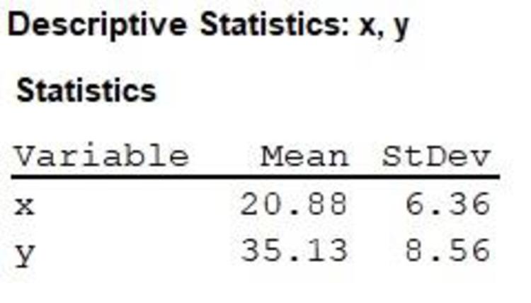
Step-by-step procedure to find the mean, standard deviation for x and y values using MINITAB is given below:
- • Choose Stat > Basic Statistics > Display
Descriptive Statistics . - • In Variables enter the columns of y and x.
- • Choose Options Statistics, select Mean and Standard deviation.
- • Click OK.
Output obtained from MINITAB is given below:
Correlation:
Where,
n represents the sample size.
The table shows the calculation of correlation:
| x | y | | ||||
| 25 | 40 | 4.12 | 4.87 | 0.6478 | 0.56893 | 0.36855 |
| 13 | 20 | –7.88 | –15.13 | –1.239 | –1.7675 | 2.18995 |
| 16 | 33 | –4.88 | –2.13 | –0.7673 | –0.2488 | 0.19093 |
| 19 | 30 | –1.88 | –5.13 | –0.2956 | –0.5993 | 0.17715 |
| 29 | 50 | 8.12 | 14.87 | 1.27673 | 1.73715 | 2.21787 |
| 19 | 37 | –1.88 | 1.87 | –0.2956 | 0.21846 | –0.0646 |
| 16 | 34 | –4.88 | –1.13 | –0.7673 | –0.132 | 0.10129 |
| 30 | 37 | 9.12 | 1.87 | 1.43396 | 0.21846 | 0.31326 |
| Total | 5.4944 |
Thus, the correlation is
Substitute r as 0.7850,
Thus, the slope
Intercept of
Substitute
Thus, the intercept
b.
Construct the 95% confidence interval for
b.
Answer to Problem 15CQ
The 95% confidence interval for
Explanation of Solution
Calculation:
The confidence interval for
Where,
Critical value:
Software procedure:
Step-by-step procedure to find the critical value using MINITAB is given below:
- • Choose Graph > Probability Distribution Plot choose View Probability > OK.
- • From Distribution, choose ‘t’ distribution.
- • In Degrees of freedom, enter 6.
- • Click the Shaded Area tab.
- • Choose Probability and Two tail for the region of the curve to shade.
- • Enter the Probability value as 0.05.
- • Click OK.
Output obtained from MINITAB is given below:
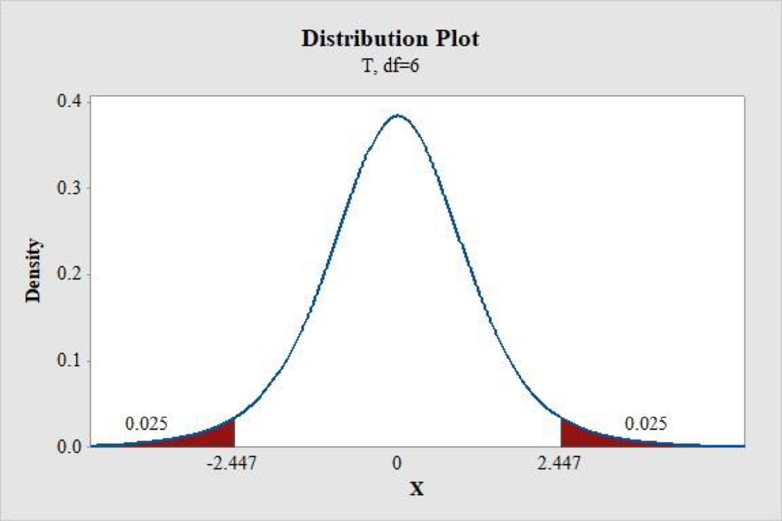
Thus, the critical value for a 95% confidence interval of
The standard error of
Where,
Calculation of residual standard deviation:
Use the estimated regression equation to find the predicted value of y for each value of x and the estimated regression equation is
The table below shows the calculation of residual standard deviation:
| x | y | |||
| 25 | 40 | 39.5 | 0.5 | 0.25 |
| 13 | 20 | 26.78 | –6.78 | 45.9684 |
| 16 | 33 | 29.96 | 3.04 | 9.2416 |
| 19 | 30 | 33.14 | -3.14 | 9.8596 |
| 29 | 50 | 43.74 | 6.26 | 39.1876 |
| 19 | 37 | 33.14 | 3.86 | 14.8996 |
| 16 | 34 | 29.96 | 4.04 | 16.3216 |
| 30 | 37 | 44.8 | –7.8 | 60.84 |
| Total | 196.57 |
Substitute
Thus, the residual standard deviation
The table shows the calculation of sum of squares for x.
| x | ||
| 25 | 4.12 | 16.9744 |
| 13 | –7.88 | 62.0944 |
| 16 | –4.88 | 23.8144 |
| 19 | –1.88 | 3.5344 |
| 29 | 8.12 | 65.9344 |
| 19 | –1.88 | 3.5344 |
| 16 | –4.88 | 23.8144 |
| 30 | 9.12 | 83.1744 |
| Total | 282.88 |
Substitute
Thus, the standard error of
95% confidence interval for
Thus, the 95% confidence interval for
c.
Test the significance of
c.
Answer to Problem 15CQ
There is no support of evidence to conclude that there is a linear relationship between x and y at 1% level of significance.
Explanation of Solution
Calculation:
The hypotheses used for testing the significance is given below:
Null hypothesis:
That is, there is no linear relationship between x and y.
Alternate hypothesis:
That is, there is a linear relationship between x and y.
Test statistic:
Where,
Substitute
Critical value:
Software procedure:
Step-by-step procedure to find the critical value using MINITAB is given below:
- • Choose Graph > Probability Distribution Plot choose View Probability > OK.
- • From Distribution, choose ‘t’ distribution.
- • In Degrees of freedom, enter 6.
- • Click the Shaded Area tab.
- • Choose Probability and Two tail for the region of the curve to shade.
- • Enter the Probability value as 0.01.
- • Click OK.
Output obtained from MINITAB is given below:
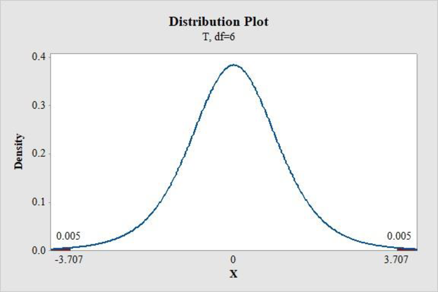
Thus, the critical value for a 99% confidence interval of
Decision Rule:
Reject the null hypothesis when the test statistic value is greater than the critical value for a given level of significance. Otherwise, do not reject the null hypothesis.
Conclusion:
The test statistic value is 3.12 and the critical value is 3.707.
The test statistic value is lesser than the critical value.
That is,
Thus, the null hypothesis is not rejected.
Hence, there is no support of evidence to conclude that there is a linear relationship between x and y at 1% level of significance.
d.
Construct the 95% confidence interval for the mean response for the given value of x.
d.
Answer to Problem 15CQ
The 95% confidence interval for the mean response for the given value of x is
Explanation of Solution
Calculation:
The given value of x is 20.
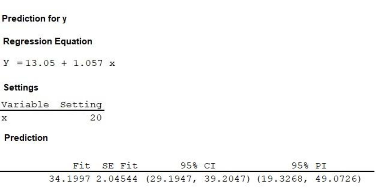
Software procedure:
Step-by-step procedure to construct the 95% confidence interval for the mean response for the given value of x is given below:
- • Choose Stat > Regression > Regression.
- • In Response, enter the column containing the y.
- • In Predictors, enter the columns containing the x.
- • Click OK.
- • Choose Stat > Regression > Regression>Predict.
- • Choose Enter the individual values.
- • Enter the x as 20.
- • Click OK.
Output obtained from MINITAB is given below:
Interpretation:
Thus, the 95% confidence interval for the mean response for the given value of x is
e.
Construct the 95% prediction interval for the individual response for the given value of x.
e.
Answer to Problem 15CQ
The 95% prediction interval for the individual response for the given value of x is
Explanation of Solution
The given value of x is 20.
From the MINITAB output obtained in the previous part (d) it can be observed that the 95% prediction interval for the individual response for the given value of x is
Want to see more full solutions like this?
Chapter 11 Solutions
Essential Statistics

 MATLAB: An Introduction with ApplicationsStatisticsISBN:9781119256830Author:Amos GilatPublisher:John Wiley & Sons Inc
 Probability and Statistics for Engineering and th...StatisticsISBN:9781305251809Author:Jay L. DevorePublisher:Cengage Learning
 Statistics for The Behavioral Sciences (MindTap C...StatisticsISBN:9781305504912Author:Frederick J Gravetter, Larry B. WallnauPublisher:Cengage Learning
 Elementary Statistics: Picturing the World (7th E...StatisticsISBN:9780134683416Author:Ron Larson, Betsy FarberPublisher:PEARSON
 The Basic Practice of StatisticsStatisticsISBN:9781319042578Author:David S. Moore, William I. Notz, Michael A. FlignerPublisher:W. H. Freeman
 Introduction to the Practice of StatisticsStatisticsISBN:9781319013387Author:David S. Moore, George P. McCabe, Bruce A. CraigPublisher:W. H. Freeman