
Videos
Here’s one to sink your teeth into: The authors of the article “Analysis of Food Crushing Sounds During Mastication: Total Sound Level Studies” (Journal of Texture Studies [1990]: 165–178) studied the nature of sounds generated during eating. Peak loudness (in decibels at 20 cm away) was measured for both open-mouth and closed-mouth chewing of potato chips and of tortilla chips. Forty subjects participated, with ten assigned at random to each combination of conditions (such as closed-mouth potato chip, and so on). We are not making this up! Summary values taken from plots given in the article appear in the accompanying table. For purposes of this exercise, suppose that it is reasonable to regard the peak loudness distributions as approximately normal.
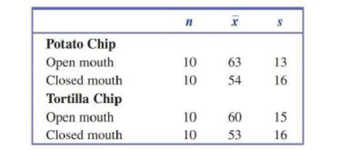
- a. Construct a 95% confidence interval tor the (inference in mean peak loudness between open-mouth and closed-mouth chewing of potato chips. Interpret the resulting interval.
- b. For closed-mouth chewing (the recommended method!), is there sufficient evidence to indicate that there is a difference between potato chips and tortilla chips with respect to mean peak loudness? Test the relevant hypotheses using α = 0.01.
- c. The means and standard deviations given here were actually for stale chips. When ten measurements of peak loudness were recorded for closed-mouth chewing of fresh tortilla chips, the resulting mean and standard deviation were 56 and 14, respectively. Is there sufficient evidence to conclude that chewing fresh tortilla chips is louder than chewing stale chips? Use α = 0.05.

Trending nowThis is a popular solution!

Chapter 11 Solutions
Introduction To Statistics And Data Analysis


- Listed below are amounts of strontium-90 (in millibecquerels, or mBq) in a simple random sample of baby teeth obtained from residents in a region born after 1979. Use the given data to construct a boxplot and identify the 5-number summary. 129 132 135 140 141 145 148 151 154 157 159 159 161 164 165 170 173 173 175 182 The 5-number summary is nothing, nothing, nothing, nothing, and nothing, all in mBq. (Use ascending order. Type integers or decimals. Do not round.)arrow_forwardResearchers interested in lead exposure due to car exhaust sampled the blood of 52 police officers subjected to constant inhalation of automobile exhaust fumes while working traffic enforcement in a primarily urban environment. The blood samples of these officers had an average lead concentration of 124.32 µg/l and a SD of 37.74 µg/l; a previous study of individuals from a nearby suburb, with no history of exposure, found an average blood level concentration of 35 µg/l. Test the hypothesis that the downtown police officers have a higher lead exposure than the group in the previous study. Interpret your results in context. Based on your preceding result, without performing a calculation, would a 99% confidence interval for the average blood concentration level of police officers contain 35 µg/l? Based on your preceding result, without performing a calculation, would a 99% confidence interval for this difference contain 0? Explain why or why not.arrow_forwardrofessor Cornish studied rainfall cycles and sunspot cycles. (Reference: Australian Journal of Physics, Vol. 7, pp. 334-346.) Part of the data include amount of rain (in mm) for 6-day intervals. The following data give rain amounts for consecutive 6-day intervals at Adelaide, South Australia. 7 28 7 1 69 3 1 4 22 7 16 4 54 160 60 73 27 3 3 1 7 144 107 4 91 44 1 8 4 22 4 59 116 52 4 155 42 24 11 43 3 24 19 74 26 63 110 39 34 71 52 39 8 0 15 2 14 9 1 2 4 9 6 10 (i) Find the median. (Use 1 decimal place.)(ii) Convert this sequence of numbers to a sequence of symbols A and B, where A indicates a value above the median and B a value below the median. Test the sequence for randomness about the median at the 5% level of significance. (b) Find the number of runs R, n1, and n2. Let n1 = number of values above the median and n2 = number of values below the median. R n1 n2 (c) In the case, n1 > 20, we cannot use Table 10 of Appendix II to find the critical…arrow_forward
- How sensitive to changes in water temperature are coral reefs? To find out, scientists examined data on sea surface temperatures, in degrees Celsius, and mean coral growth, in centimeters per year, over a several‑year period at locations in the Gulf of Mexico and the Caribbean Sea. The table shows the data for the Gulf of Mexico. Sea surface temperature 26.726.7 26.626.6 26.626.6 26.526.5 26.326.3 26.126.1 Growth 0.850.85 0.850.85 0.790.79 0.860.86 0.890.89 0.920.92 (b) Find the correlation ?r step by step. Round off to two decimals places in each step. First, find the mean and standard deviation of each variable. Then, find the six standardized values for each variable. Finally, use the formula for ?r . Round your answer to three decimal places.arrow_forwardA fisheries biologist collected a random sample of fish from a lake and conducted a chi-square goodness-of-fit test to see if the distribution of fish changed over time. The table below shows the distribution of fish that were put into the lake when it was originally stocked. Fish Type Trout Bass Perch Sunfish Catfish Percent 25% 25% 20% 15% 15% The biologist found evidence to reject the null hypothesis in favor of the alternative hypothesis. Which of the following represents the alternative hypothesis of the test?arrow_forwardThe data in the accompanying table are from a paper. Suppose that each person in a random sample of 49 male students and in a random sample of 88 female students at a particular college was classified according to gender and whether they usually or rarely eat three meals a day. Find the test statistic and P-value. (Use SALT. Round your test statistic to three decimal places and your P-value to four decimal places.) Usually Eat3 Meals a Day Rarely Eat3 Meals a Day Male 26 23 Female 35 53arrow_forward
- In an experiment to determine the effect of ambient temperature on the emissons of oxides of nitrogen ( NOx ) of diesel trucks, 10 trucks were run at temperatures of 40°F and 80°F . The emissions, in parts per billion, are presented in the following table. Truck 40°F 80°F 1 926.5 896.7 2 851.1 857.0 3 975.5 952.1 4 1009.3 884.8 5 871.8 840.7 6 949.2 885.1 7 1006.3 885.5 8 836.5 777.8 9 837.8 850.2 10 958.9 882.1 Send data to Excel Let μ1 represent the mean emission at 40°F and =μd−μ1μ2 .Can you conclude that the mean emission differs between the two temperatures? Use the =α0.05 level of significance and the TI-84 Plus calculator to answer the following. p value ? do we reject? is there enough evidence :?arrow_forwardA paper investigated the driving behavior of teenagers by observing their vehicles as they left a high school parking lot and then again at a site approximately 1 2 mile from the school. Assume that it is reasonable to regard the teen drivers in this study as representative of the population of teen drivers. Amount by Which Speed Limit Was Exceeded MaleDriver FemaleDriver 1.2 -0.1 1.4 0.4 0.9 1.1 2.1 0.7 0.7 1.1 1.3 1.2 3 0.1 1.3 0.9 0.6 0.5 2.1 0.5 (a) Use a .01 level of significance for any hypothesis tests. Data consistent with summary quantities appearing in the paper are given in the table. The measurements represent the difference between the observed vehicle speed and the posted speed limit (in miles per hour) for a sample of male teenage drivers and a sample of female teenage drivers. (Use μmales − μfemales.Round your test statistic to two decimal places. Round your degrees of freedom down to the nearest whole number. Round your p-value to…arrow_forwardA paper investigated the driving behavior of teenagers by observing their vehicles as they left a high school parking lot and then again at a site approximately 1 2 mile from the school. Assume that it is reasonable to regard the teen drivers in this study as representative of the population of teen drivers. Amount by Which Speed Limit Was Exceeded MaleDriver FemaleDriver 1.3 -0.1 1.3 0.4 0.9 1.1 2.1 0.7 0.7 1.1 1.3 1.2 3 0.1 1.3 0.9 0.6 0.5 2.1 0.5 (a) Use a .01 level of significance for any hypothesis tests. Data consistent with summary quantities appearing in the paper are given in the table. The measurements represent the difference between the observed vehicle speed and the posted speed limit (in miles per hour) for a sample of male teenage drivers and a sample of female teenage drivers. (Use μmales − μfemales.Round your test statistic to two decimal places. Round your degrees of freedom down to the nearest whole number. Round your p-value to…arrow_forward
- An article in the Journal of Applied Polymer Science (Vol. 56, pp. 471–476, 1995) studied the effect of the mole ratio of sebacic acid on the intrinsic viscosity of copolyesters.- The data follows: Viscosity 0.45 0.2 0.34 0.58 0.7 0.57 0.55 0.44 Mole ratio 1 0.9 0.8 0.7 0.6 0.5 0.4 0.3 (a) Construct a scatter diagram of the data.arrow_forwardBased on data collected by the U.S. General Social Survey, a researcher examines the frequency with which adults responded to two questions. The first asked people if they resided in the same city or town now as when they were 16 years old (Residence). The second asked if they found life generally exciting, routine, or dull (Life). Using data from 2,791 people, the results are below. Life is Generally: Living in: Exciting Routine Dull Marginal n Same City or Town O = 489 E = O = 601 E = O = 64 E = 1154 Different Area O = 797 E = O = 763 E = O = 77 E = 1637 Marginal n 1286 1364 141 2791 Using the chi-square (χ2) test for independence, examine if the feelings people have about life in general are related to living in the same city or town as when a teen. State the hypotheses (H0 and H1). Find the critical value for α = .05, 1-tailed. Calculate the test statistic (χ2), filling in relevant portions of the…arrow_forwardHow sensitive to changes in water temperature are coral reefs? To find out, scientists examined data on sea surface temperatures and coral growth per year at locations in the Gulf of Mexico and the Caribbean Sea. The table shows the data for the Gulf of Mexico. Sea surface temperature 26.726.7 26.626.6 26.626.6 26.526.5 26.326.3 26.126.1 Growth 0.850.85 0.850.85 0.790.79 0.860.86 0.890.89 0.920.92 Click to download the data in your preferred format. CSV Excel JMP Mac-Text Minitab14-18 Minitab18+ PC-Text R SPSS TI CrunchIt! © Macmillan Learning (a) Make a scatterplot. Which is the explanatory variable? The plot shows a negative linear pattern. Explanatory Variable: How sensitive to changes in water temperature are coral reefs? To find out, scientists examined data on sea surface temperatures and coral growth per year at locations in the Gulf of Mexico and the Caribbean Sea. The table shows the data…arrow_forward
 Glencoe Algebra 1, Student Edition, 9780079039897...AlgebraISBN:9780079039897Author:CarterPublisher:McGraw Hill