
Concept explainers
Videos
a.
Calculate the values of
a.
Answer to Problem 43E
The value of
The value of
The value of
The value of
Explanation of Solution
Calculation:
The number of years of service (x) and the hourly wages ($) (y) of the five employees of a small company are given.
Denote
Software procedure:
Step-by-step procedure to obtain the descriptive statistics using the MINITAB software:
- Choose Stat > Basic Statistics > Display Descriptive Statistics, click OK.
- In Variables, enter the columns of x and y.
- Choose Statistics, select Mean, Standard deviation and click OK.
- Click OK.
Output using the MINITAB software is given below:
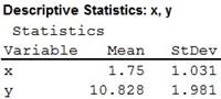
From the above output, it is evident that the value of
b.
Find the
b.
Answer to Problem 43E
The
Explanation of Solution
Calculation:
Correlation:
The correlation coefficient, r, between ordered pairs of variables, (x, y) having sample means
Software procedure:
Step-by-step procedure to obtain the correlation using the MINITAB software:
- Choose Stat > Basic Statistics > Correlation.
- In Variables, enter the columns of x and y.
- Click OK.
Output using the MINITAB software is given below:
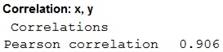
From the output, the correlation coefficient between the years of service and the hourly wages is 0.906.
c.
Find the sample mean and the sample standard deviation of the hourly wages, if each employee is given a raise of $1.00 per hour.
c.
Answer to Problem 43E
The sample mean of the hourly wages, if each employee is given a raise of $1.00 per hour is 11.828.
The sample standard deviation of the hourly wages, if each employee is given a raise of $1.00 per hour is 1.981.
Explanation of Solution
Calculation:
Denote
The calculation for
| y | |
| 9.50 | 10.50 |
| 8.23 | 9.23 |
| 10.95 | 11.95 |
| 12.70 | 13.70 |
| 12.75 | 13.75 |
Descriptive statistics:
Software procedure:
Step-by-step procedure to obtain the descriptive statistics using the MINITAB software:
- Choose Stat > Basic Statistics > Display Descriptive Statistics, click OK.
- In Variables, enter the columns of y1.
- Choose Statistics, select Mean, Standard deviation and click OK.
- Click OK.
Output using the MINITAB software is given below:
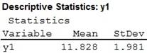
From the above output, it is evident that the sample mean of the hourly wages, if each employee is given a raise of $1.00 per hour is 11.828 and the sample standard deviation of the hourly wages, if each employee is given a raise of $1.00 per hour is 1.981.
d.
Identify the effects of increasing each value of y by 1 on the values of
d.
Answer to Problem 43E
The average hourly wage
The standard deviation
Explanation of Solution
Interpretation:
From part a, the value of average hourly wages,
From part c, the value of sample mean of the hourly wages, if each employee is given a raise of $1.00 per hour is 11.828.
Now,
Hence, it is evident that the average hourly wage has increased by $1.00 due to increasing each value of y by 1.
From part a, the value of standard deviation of hourly wages,
From part c, the value of sample standard deviation , if each employee is given a raise of $1.00 per hour is 1.981.
Evidently, the standard deviation has remained unchanged due to increasing each value of y by 1.
e.
Find the correlation coefficient between the years of service and the increased hourly wages.
Explain the reason the correlation coefficient remains unchanged even when the values of y change.
e.
Answer to Problem 43E
The correlation coefficient between the years of service and the increased hourly wages is 0.906.
Explanation of Solution
Calculation:
Correlation:
Software procedure:
Step-by-step procedure to obtain the correlation using the MINITAB software:
- Choose Stat > Basic Statistics > Correlation.
- In Variables, enter the columns of x and y1.
- Click OK.
Output using the MINITAB software is given below:
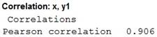
From the output, the correlation coefficient between the years of service and the increased hourly wages is 0.906.
Consider the formula for the correlation coefficient, r:
Now, each y increases and becomes
Again, as observed from part d, the mean of the increased hourly wages is
Replace these in the formula for the correlation coefficient:
It is observed that the correlation coefficient is independent of the change of origin.
Hence, the correlation coefficient remains unchanged even when the values of y change.
f.
Find the sample mean and the sample standard deviation of the service period, if it is expressed in terms of months.
f.
Answer to Problem 43E
The sample mean of the hourly wages, of the service period, if it is expressed in terms of months is 21.
The sample standard deviation of the hourly wages, of the service period, if it is expressed in terms of months is 12.37.
Explanation of Solution
Calculation:
Denote
The calculation for
| x | |
| 0.5 | 6 |
| 1.0 | 12 |
| 1.75 | 21 |
| 2.5 | 30 |
| 3.0 | 36 |
Descriptive statistics:
Software procedure:
Step-by-step procedure to obtain the descriptive statistics using the MINITAB software:
- Choose Stat > Basic Statistics > Display Descriptive Statistics, click OK.
- In Variables, enter the columns of x1.
- Choose Statistics, select Mean, Standard deviation and click OK.
- Click OK.
Output using the MINITAB software is given below:
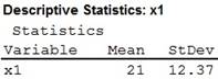
From the above output, it is evident that the sample mean of the hourly wages, of the service period, if it is expressed in terms of months is 21 and the sample standard deviation of the hourly wages, of the service period, if it is expressed in terms of months is 12.37.
g.
Identify the effects of multiplying each value of x by 12 on the values of
g.
Answer to Problem 43E
The average service period in months has been multiplied by 12 due to multiplying each value of x by 12.
The standard deviation has been multiplied by 12 due to multiplying each value of x by 12.
Explanation of Solution
Interpretation:
From part a, the average service period in years,
From part f, the average service period in months is 21.
Now,
Hence, it is evident that the average hourly wage has increased by $1.00 due to increasing each value of y by 1.
From part a, the value of standard deviation of service period in years,
From part c, the value of sample standard deviation of service period in months is 12.37.
Now,
In other words,
Evidently, the standard deviation has been multiplied by 12 due to multiplying each value of x by 12.
h.
Find the correlation coefficient between the months of service and the hourly wages.
Explain the reason the correlation coefficient remains unchanged even when the values of
h.
Answer to Problem 43E
The correlation coefficient between the months of service and the increased hourly wages is 0.906.
Explanation of Solution
Calculation:
Correlation:
Software procedure:
Step-by-step procedure to obtain the correlation using the MINITAB software:
- Choose Stat > Basic Statistics > Correlation.
- In Variables, enter the columns of x1 and y.
- Click OK.
Output using the MINITAB software is given below:
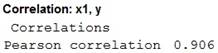
From the output, the correlation coefficient between the months of service and the increased hourly wages is 0.906.
Consider the formula for the correlation coefficient, r:
Now, each x is multiplied by 12 and becomes
Again, as observed from part d, the mean of the months of service is
Replace these in the formula for the correlation coefficient:
It is observed that the correlation coefficient is independent of the changes of origin and scale.
Hence, the correlation coefficient remains unchanged even when the values of
i.
Find the effect of adding a constant to each x-value or to each y-value on the correlation coefficient.
i.
Answer to Problem 43E
If a constant is added to each x-value or to each y-value, the correlation coefficient is unchanged.
Explanation of Solution
Interpretation:
The correlation coefficient is independent of the change of origin of the variables. Adding a constant to each x-value or to each y-value implies a change in origin of x or y.
Hence, if a constant is added to each x-value or to each y-value, the correlation coefficient is unchanged.
Correlation:
The correlation coefficient, r, between ordered pairs of variables, (x, y) having sample means
j.
Find the effect of multiplying a positive constant to each x-value or to each y-value on the correlation coefficient.
j.
Answer to Problem 43E
If each x-value or each y-value is multiplied by a positive constant, the correlation coefficient is unchanged.
Explanation of Solution
Interpretation:
The correlation coefficient is independent of the change of scale of the variables. Multiplying a positive constant with each x-value or each y-value changes the scale of x or y.
Hence, if each x-value or each y-value is multiplied by a positive constant, the correlation coefficient is unchanged.
Want to see more full solutions like this?
Chapter 11 Solutions
Essential Statistics


 MATLAB: An Introduction with ApplicationsStatisticsISBN:9781119256830Author:Amos GilatPublisher:John Wiley & Sons Inc
 Probability and Statistics for Engineering and th...StatisticsISBN:9781305251809Author:Jay L. DevorePublisher:Cengage Learning
 Statistics for The Behavioral Sciences (MindTap C...StatisticsISBN:9781305504912Author:Frederick J Gravetter, Larry B. WallnauPublisher:Cengage Learning
 Elementary Statistics: Picturing the World (7th E...StatisticsISBN:9780134683416Author:Ron Larson, Betsy FarberPublisher:PEARSON
 The Basic Practice of StatisticsStatisticsISBN:9781319042578Author:David S. Moore, William I. Notz, Michael A. FlignerPublisher:W. H. Freeman
 Introduction to the Practice of StatisticsStatisticsISBN:9781319013387Author:David S. Moore, George P. McCabe, Bruce A. CraigPublisher:W. H. Freeman