
Mathematical Statistics with Applications
7th Edition
ISBN: 9781133384380
Author: Dennis Wackerly; William Mendenhall; Richard L. Scheaffer
Publisher: Cengage Learning US
expand_more
expand_more
format_list_bulleted
Concept explainers
Videos
Textbook Question
Chapter 11.6, Problem 39E
Refer to Exercise 11.16. Find a 95% confidence interval for the mean potency of a 1-ounce portion of antibiotic stored at 65°F.
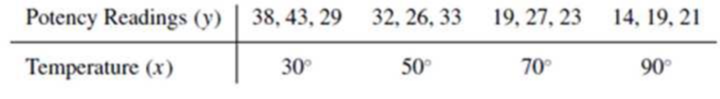
11.16 An experiment was conducted to observe the effect of an increase in temperature on the potency of an antibiotic. Three 1-ounce portions of the antibiotic were stored for equal lengths of time at each of the following Fahrenheit temperatures: 30°, 50°, 70°, and 90°. The potency readings observed at the end of the experimental period were as shown in the following table.
- a Find the least-squares line appropriate for this data.
- b Plot the points and graph the line as a check on your calculations.
- c Calculate S2.
Expert Solution & Answer
Want to see the full answer?
Check out a sample textbook solution
Students have asked these similar questions
A study of runoff water from a manufacturing plant was made. Included in the study were pH measurements for six water specimens: 5.9, 5.0, 6.5, 5.6, 5.9, 6.5. Assume that these are a random sample of water specimens from a normal population. A 98% prediction interval for a pH of a single specimen is closest to
Unfortunately, arsenic occurs naturally in some ground water.t A mean arsenic level of u = 8.0 parts per billion (ppb) is considered safe for agricultural use. A well in Texas is used to water cotton crops.
This well is tested on a regular basis for arsenic. A random sample of 36 tests gave a sample mean of x = 6.7 ppb arsenic, with s = 3.0 ppb. Does this information indicate that the mean level of arsenic
in this well is less than 8 ppb? Use a = 0.01.
n USE SALT
(a) What is the level of significance?
State the null and alternate hypotheses.
O Ho: H = 8 ppb; H,: u > 8 ppb
O Ho: H = 8 ppb; H,: H + 8 ppb
O Ho: H 8 ppb; H,: u = 8 ppb
O Ho: H = 8 ppb; H,: µ 0.100
O 0.050 < P-value < 0.100
O 0.010 < P-value < 0.050
O 0.005 < P-value < 0.010
P-value < 0.005
Sketch the sampling distribution and show the area corresponding to the P-value.
MacBook Pro
esc
Unfortunately, arsenic occurs naturally in some ground water.t A mean arsenic level of u = 8.0 parts per billion (ppb) is
considered safe for agricultural use. A well in Texas is used to water cotton crops. This well is tested on a regular basis for arsenic.
A random sample of 36 tests gave a sample mean of x = 7.1 ppb arsenic, with s = 2.2 ppb. Does this information indicate that
the mean level of arsenic in this well is less than 8 ppb? Use a = 0.01.
A USE SALT
(a) What is the level of significance?
State the null and alternate hypotheses.
O Ho: H= 8 ppb; H,: H > 8 ppb
O Ho: H 8 ppb; H: H = 8 ppb
(b) What sampling distribution will you use? Explain the rationale for your choice of sampling distribution.
O The standard normal, since the sample size is large and a is unknown.
O The Student's t, since the sample size is large and a is known.
O The standard normal, since the sample size is large and a is known.
O The Student's t, since the sample size is large and a is unknown.
What is…
Chapter 11 Solutions
Mathematical Statistics with Applications
Ch. 11.3 - If 0 and 1 are the least-squares estimates for the...Ch. 11.3 - Prob. 2ECh. 11.3 - Fit a straight line to the five data points in the...Ch. 11.3 - Auditors are often required to compare the audited...Ch. 11.3 - Prob. 5ECh. 11.3 - Applet Exercise Refer to Exercises 11.2 and 11.5....Ch. 11.3 - Prob. 7ECh. 11.3 - Laboratory experiments designed to measure LC50...Ch. 11.3 - Prob. 9ECh. 11.3 - Suppose that we have postulated the model...
Ch. 11.3 - Some data obtained by C.E. Marcellari on the...Ch. 11.3 - Processors usually preserve cucumbers by...Ch. 11.3 - J. H. Matis and T. E. Wehrly report the following...Ch. 11.4 - a Derive the following identity:...Ch. 11.4 - An experiment was conducted to observe the effect...Ch. 11.4 - Prob. 17ECh. 11.4 - Prob. 18ECh. 11.4 - A study was conducted to determine the effects of...Ch. 11.4 - Suppose that Y1, Y2,,Yn are independent normal...Ch. 11.4 - Under the assumptions of Exercise 11.20, find...Ch. 11.4 - Prob. 22ECh. 11.5 - Use the properties of the least-squares estimators...Ch. 11.5 - Do the data in Exercise 11.19 present sufficient...Ch. 11.5 - Use the properties of the least-squares estimators...Ch. 11.5 - Let Y1, Y2, . . . , Yn be as given in Exercise...Ch. 11.5 - Prob. 30ECh. 11.5 - Using a chemical procedure called differential...Ch. 11.5 - Prob. 32ECh. 11.5 - Prob. 33ECh. 11.5 - Prob. 34ECh. 11.6 - For the simple linear regression model Y = 0 + 1x...Ch. 11.6 - Prob. 36ECh. 11.6 - Using the model fit to the data of Exercise 11.8,...Ch. 11.6 - Refer to Exercise 11.3. Find a 90% confidence...Ch. 11.6 - Refer to Exercise 11.16. Find a 95% confidence...Ch. 11.6 - Refer to Exercise 11.14. Find a 90% confidence...Ch. 11.6 - Prob. 41ECh. 11.7 - Suppose that the model Y=0+1+ is fit to the n data...Ch. 11.7 - Prob. 43ECh. 11.7 - Prob. 44ECh. 11.7 - Prob. 45ECh. 11.7 - Refer to Exercise 11.16. Find a 95% prediction...Ch. 11.7 - Refer to Exercise 11.14. Find a 95% prediction...Ch. 11.8 - The accompanying table gives the peak power load...Ch. 11.8 - Prob. 49ECh. 11.8 - Prob. 50ECh. 11.8 - Prob. 51ECh. 11.8 - Prob. 52ECh. 11.8 - Prob. 54ECh. 11.8 - Prob. 55ECh. 11.8 - Prob. 57ECh. 11.8 - Prob. 58ECh. 11.8 - Prob. 59ECh. 11.8 - Prob. 60ECh. 11.9 - Refer to Example 11.10. Find a 90% prediction...Ch. 11.9 - Prob. 62ECh. 11.9 - Prob. 63ECh. 11.9 - Prob. 64ECh. 11.9 - Prob. 65ECh. 11.10 - Refer to Exercise 11.3. Fit the model suggested...Ch. 11.10 - Prob. 67ECh. 11.10 - Fit the quadratic model Y=0+1x+2x2+ to the data...Ch. 11.10 - The manufacturer of Lexus automobiles has steadily...Ch. 11.10 - a Calculate SSE and S2 for Exercise 11.4. Use the...Ch. 11.12 - Consider the general linear model...Ch. 11.12 - Prob. 72ECh. 11.12 - Prob. 73ECh. 11.12 - An experiment was conducted to investigate the...Ch. 11.12 - Prob. 75ECh. 11.12 - The results that follow were obtained from an...Ch. 11.13 - Prob. 77ECh. 11.13 - Prob. 78ECh. 11.13 - Prob. 79ECh. 11.14 - Prob. 80ECh. 11.14 - Prob. 81ECh. 11.14 - Prob. 82ECh. 11.14 - Prob. 83ECh. 11.14 - Prob. 84ECh. 11.14 - Prob. 85ECh. 11.14 - Prob. 86ECh. 11.14 - Prob. 87ECh. 11.14 - Prob. 88ECh. 11.14 - Refer to the three models given in Exercise 11.88....Ch. 11.14 - Prob. 90ECh. 11.14 - Prob. 91ECh. 11.14 - Prob. 92ECh. 11.14 - Prob. 93ECh. 11.14 - Prob. 94ECh. 11 - At temperatures approaching absolute zero (273C),...Ch. 11 - A study was conducted to determine whether a...Ch. 11 - Prob. 97SECh. 11 - Prob. 98SECh. 11 - Prob. 99SECh. 11 - Prob. 100SECh. 11 - Prob. 102SECh. 11 - Prob. 103SECh. 11 - An experiment was conducted to determine the...Ch. 11 - Prob. 105SECh. 11 - Prob. 106SECh. 11 - Prob. 107SE
Knowledge Booster


Learn more about
Need a deep-dive on the concept behind this application? Look no further. Learn more about this topic, statistics and related others by exploring similar questions and additional content below.Similar questions
- Unfortunately, arsenic occurs naturally in some ground water.t A mean arsenic level of u = 8.0 parts per billion (ppb) is considered safe for agricultural use. A well in Texas is used to water cotton crops. This well is tested on a regular basis for arsenic. A random sample of 36 tests gave a sample mean of x = 7.1 ppb arsenic, with s = 2.2 ppb. Does this information indicate that the mean level of arsenic in this well is less than 8 ppb? Use a = 0.01. A USE SALT (a) What is the level of significance? State the null and alternate hypotheses. O Họ: u = 8 ppb; H,: u > 8 ppb O Ho: H 8 ppb; H,: u = 8 ppb (b) What sampling distribution will you use? Explain the rationale for your choice of sampling distribution. The standard normal, since the sample size is large and a is unknown. O The Student's t, since the sample size is large and a is known. O The standard normal, since the sample size is large and a is known. The Student's t, since the sample size is large and a is unknown. What is the…arrow_forwardA random sample of 150 individuals (males and females) was surveyed, and the individuals were asked to indicate their year incomes. The results of the survey are shown below. Income Category Category 1: $20,000 up to $40,000 Category 2: $40,000 up to $60,000 Category 3: $60,000 up to $80,000 Edit Format Table Test at a = .05 to determine if the yearly income is independent of the gender. (CSLO 1,6,7) 12pt Male 10 35 15 V Paragraph BI U A Female 30 15 45 > 2 T² :arrow_forwardTwo random samples of 32 individuals were chosen. The average breathing rate of the first sample was 21 breaths per minute after jogging for twenty minutes, and the average breathing rate of the second sample was 19 breaths per minute after walking for twenty minutes. If the population standard deviation is 4.2 breaths per minute for jogging and 4.5 breaths per minute for walking, test the claim that the breathing rate for jogging is more than the breathing rate for walking. Assume a = 0.055. Let the breathing rates of joggers represent population 1 and the breathing rate of walkers represent population 2. a.) State the null and alternative hypothesis using correct symbolic form. Ho: 1 → f₂ H₁ H1 2 b.) What is the critical value? (round to two decimal places) Z=arrow_forward
- Refer to the data presented in Exercise 2.86. Note that there were 50% more accidents in the 25 to less than 30 age group than in the 20 to less than 25 age group. Does this suggest that the older group of drivers in this city is more accident- prone than the younger group? What other explanation might account for the difference in accident rates?arrow_forwardYou are a correctional officer interested in whether the 45 children in your juvenile facility have significantly different recidivism rates than the population of juveniles in correctional facilities. The recidivism for your 45 children is an average of 14 per year (standard deviation of 2). The population recidivism has an average of 10 per year. The alpha level is .05. What is the t-calculated?arrow_forwardScores on an accounting exam ranged from 42 to 92, with quartiles Q1= 59.00, Q2= 79.0, and Q3=82.25. %3Darrow_forward
- The mean number of close friends for the population freshman college students in the U.S.A. is u 5.7. The standard deviation of scores in this population is 1.3. A psychologist predicts that the mean number of close friends for freshman introverts will be significantly different from the mean of the population. The mean number of close friends for a random sample of 25 freshman introverts is M = 6.5. Set your alpha level at a = .05. Complete steps 3 and 4 of the hypothesis testing procedure. What decision should the researcher make regarding the effect of introversion on the number of close friends? = O The researcher should retain Ho and conclude that introversion has no effect on the number of close friends. The researcher should retain HA and conclude that introversion has no effect on the number of close friends. O The researcher should reject Ho and conclude that introversion makes a difference in the number of close friends one has. O The researcher should reject HA and conclude…arrow_forwardThe United States ranks ninth in the world in per capita chocolate consumption; Forbes reports that the average American eats 9.5 pounds of chocolate annually. Suppose you are curious whether chocolate consumption is higher in Hershey, Pennsylvania, the location of the Hershey Company's corporate headquarters. A sample of 35 individuals from the Hershey area showed a sample mean annual consumption of 10.05 pounds and a standard deviation of s = 1.5 pounds. Using α = 0.05, do the sample results support the conclusion that mean annual consumption of chocolate is higher in Hershey than it is throughout the United States? State the null and alternative hypotheses. (Enter != for ≠ as needed.) H0:_________________ Ha:__________________ Find the value of the test statistic. (Round your answer to three decimal places.) _____________________. Find the p-value. (Round your answer to four decimal places.) p-value =____________________. State your conclusion.(multiple choice) A.…arrow_forwardTo compare the dry braking distances from 30 to 0 miles per hour for two makes of automobiles, a safety engineer conducts braking tests for 35 models of Make A and 35 models of Make B. The mean braking distance for Make A is 42 feet. Assume the population standard deviation is 4.5 feet. The mean braking distance for Make B is 46 feet. Assume the population standard deviation is 4.4 feet. At α=0.10, can the engineer support the claim that the mean braking distances are different for the two makes of automobiles? Assume the samples are random and independent, and the populations are normally distributed. Complete parts (a) through (e).arrow_forward
- According to a report from the United States Environmental Protection Agency, burning one gallon of gasoline typically emits about 8.9 kg of CO2. A fuel company wants to test a new type of gasoline designed to have lower CO2 emissions. Here are their hypotheses: Ho: = 8.9 kg Ha:H< 8.9 kg (where u is the mean amount of CO2 emitted by burning one gallon of this new gasoline). Under which of the following conditions would the company commit a Type I error?arrow_forwardSulfur compounds cause "off-odors" in wine, and winemakers want to know the odor threshold – the lowest concentration of a compound that the human nose can detect. The odor threshold for dimethyl sulfide (DMS) in trained wine tasters is about 25 micrograms per liter of wine (µg/L). The untrained noses of consumers may be less sensitive, however. A set of DMS odor threshold data for 10 untrained students was analyzed. How sensitive are the untrained noses of students? You want to estimate the mean DMS odor threshold among all students, and you would be satisfied to estimate the mean to within ±0.25 with 95% confidence. The standard deviation of the odor threshold for untrained noses is known to be o = 8 micrograms per liter of wine. How large an SRS of untrained students do you need? Give your answer rounded up to the nearest whole number. n = Incorrectarrow_forwardTo compare the dry braking distances from 30 to 0 miles per hour for two makes of automobiles, a safety engineer conducts braking tests for 35 models of Make A and 35 models of Make B. The mean braking distance for Make A is 43 feet. Assume the population standard deviation is 4.6 feet. The mean braking distance for Make B is 47 feet. Assume the population standard deviation is 4.2 feet. At α=0.10, can the engineer support the claim that the mean braking distances are different for the two makes of automobiles? Assume the samples are random and independent, and the populations are normally distributed. Complete parts (a) through (e).arrow_forward
arrow_back_ios
SEE MORE QUESTIONS
arrow_forward_ios
Recommended textbooks for you
 Glencoe Algebra 1, Student Edition, 9780079039897...AlgebraISBN:9780079039897Author:CarterPublisher:McGraw Hill
Glencoe Algebra 1, Student Edition, 9780079039897...
Algebra
ISBN:9780079039897
Author:Carter
Publisher:McGraw Hill
Statistics 4.1 Point Estimators; Author: Dr. Jack L. Jackson II;https://www.youtube.com/watch?v=2MrI0J8XCEE;License: Standard YouTube License, CC-BY
Statistics 101: Point Estimators; Author: Brandon Foltz;https://www.youtube.com/watch?v=4v41z3HwLaM;License: Standard YouTube License, CC-BY
Central limit theorem; Author: 365 Data Science;https://www.youtube.com/watch?v=b5xQmk9veZ4;License: Standard YouTube License, CC-BY
Point Estimate Definition & Example; Author: Prof. Essa;https://www.youtube.com/watch?v=OTVwtvQmSn0;License: Standard Youtube License
Point Estimation; Author: Vamsidhar Ambatipudi;https://www.youtube.com/watch?v=flqhlM2bZWc;License: Standard Youtube License