Chapter 12, Problem 106SE

a.

To determine

Find the missing quantities.

Answer to Problem 106SE

The filled regression analysis table is,

Predictor	Coefficient		SE Coefficient	T		P
Constant	517.46		11.76	44.0017		0
$x_1$	11.4720		0.314	36.50		0
$x_2$	–8.1378		0.1969	–41.3296		0
$x_3$	10.8565		0.6652	16.3207		0
$S=10.2560$		$\underset{\_}{\text{R-Sq}=99.5\%}$			$\underset{\_}{\text{R-Sq}\left(\text{adj}\text{.}\right)=99.4\%}$
Analysis of Variance
Source	DF		SS	MS		F	P
Regression	3		347,300	115,767		1,102.543	0
Residual Error	16		1,683	105
Total	19		348,983

Explanation of Solution

Calculation:

An incomplete regression analysis table is given.

Multiple linear regression model:

A multiple linear regression model is given as $y_i={\beta }_0+{\beta }_1{x}_{1i}+\mathrm{...}+{\beta }_k{x}_{ki}+{\epsilon }_i$ where $y_i$ is the response variable, and $x_{1i},x_{2i},\mathrm{...},x_{ki}$ are the k predictor variables. The quantities ${\beta }_0,{\beta }_1,\mathrm{...},{\beta }_k$ are the slopes corresponding to $x_{1i},x_{2i},\mathrm{...},x_{ki}$ respectively.${\widehat{\beta }}_0$ is the estimated intercept of the line, from the sample data.

The t-statistic is obtained as,

$T_0=\frac{{\widehat{\text{β}}}_j-{\text{β}}_{j0}}{se\left({\widehat{\text{β}}}_j\right)}$ where ${\widehat{\text{β}}}_j$ is the estimate of j^th coefficient, ${\text{β}}_{j0}=0$ and $se\left({\widehat{\text{β}}}_j\right)$ be the standard error of ${\widehat{\text{β}}}_j$.

The test statistic $T_0$ follows t distribution with degrees of freedom

$n-\left(k+1\right)$ where k be the number of repressor.

In the given problem the regression equation is $Y=517+11.5x_1-8.14x_2+10.9x_3$.

Hence, there are 3 regressors and $k=3$.

Now, using the given information it can be found that,

Predictor	Coefficient $\left({\widehat{\text{β}}}_j\right)$	SE Coefficient $\left(se\left({\widehat{\text{β}}}_j\right)\right)$	$T_0$
Constant	517.46	11.76	$\frac{517.46}{11.76}=44.0017$
$x_1$	11.4720	$\frac{11.4720}{36.50}=0.314$	36.50
$x_2$	–8.1378	0.1969	$\frac{-8.1378-0}{0.1969}=-41.3296$
$x_3$	10.8565	0.6652	$\frac{10.8565-0}{0.6652}=16.3207$

The total observation is 19. Thus, $n=19$.

In the given problem, the degrees of freedom for t-statistic is,

$\begin{array}{c}n-\left(k+1\right)=n-k-1\\ =19-3-1\\ =15\end{array}$

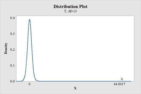
P- value:

Software procedure:

Step by step procedure to obtain the P- value using the MINITAB software is given below:

• Choose Graph > Probability Distribution Plot choose View Probability > OK.
• From Distribution, choose ‘t’ distribution.
• Enter Degree of freedom as 15.
• Click the Shaded Area tab.
• Choose X value and Right tail for the region of the curve to shade.
• Enter the X value as 44.0017.
• Click OK.

Output using the MINITAB software is given below:

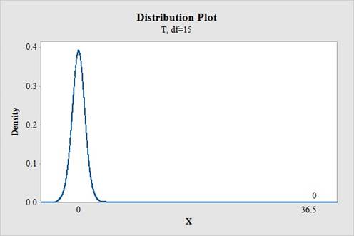
P- value:

Software procedure:

Step by step procedure to obtain the P- value using the MINITAB software is given below:

• Choose Graph > Probability Distribution Plot choose View Probability > OK.
• From Distribution, choose ‘t’ distribution.
• Enter Degree of freedom as 15.
• Click the Shaded Area tab.
• Choose X value and Right tail for the region of the curve to shade.
• Enter the X value as 36.50.
• Click OK.

Output using the MINITAB software is given below:

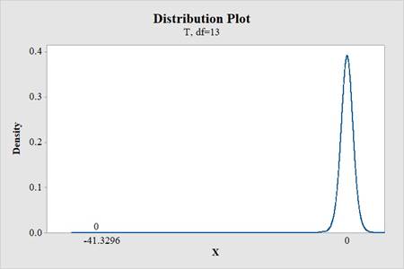
P- value:

Software procedure:

Step by step procedure to obtain the P- value using the MINITAB software is given below:

• Choose Graph > Probability Distribution Plot choose View Probability > OK.
• From Distribution, choose ‘t’ distribution.
• Enter Degree of freedom as 15.
• Click the Shaded Area tab.
• Choose X value and Left tail for the region of the curve to shade.
• Enter the X value as –41.3296.
• Click OK.

Output using the MINITAB software is given below:

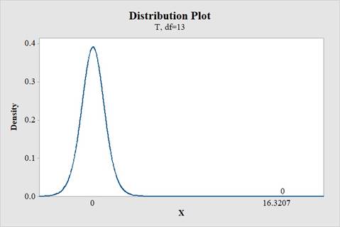
P- value:

Software procedure:

Step by step procedure to obtain the P- value using the MINITAB software is given below:

• Choose Graph > Probability Distribution Plot choose View Probability > OK.
• From Distribution, choose ‘t’ distribution.
• Enter Degree of freedom as 15.
• Click the Shaded Area tab.
• Choose X value and Right tail for the region of the curve to shade.
• Enter the X value as 16.3207.
• Click OK.

Output using the MINITAB software is given below:

Hence, the corresponding P-values are,

Predictor	$T_0$	P-value
Constant	44.0017	0
$x_1$	36.50	0
$x_2$	–41.3296	0
$x_3$	16.3207	0

The F-statistic is obtained as,

$\begin{array}{c}{F}_0=\frac{\frac{S{S}_R}{k}}{\frac{S{S}_E}{n-\left(k+1\right)}}\\ =\frac{M{S}_R}{M{S}_E}\end{array}$ , where $S{S}_R$ is the sum of square die tor regression, $S{S}_E$ sum of square due to error, $M{S}_R$ is the mean square due to regression and $M{S}_E$ is the mean square die to error for k regressors with sample size n.

The F-statistic follows F distribution with numerator degrees of freedom k and denominator degrees of freedom $n-\left(k+1\right)$.

It is also known that, $S{S}_T=S{S}_R+S{S}_E$, where $S{S}_T$ is the total sum pf square.

Now, it is given that $S{S}_T=348,983$ and $S{S}_R=347,300$.

Hence,

$\begin{array}{c}348,983=347,300+S{S}_E\\ S{S}_E=348,983-347,300\\ =1,683\end{array}$

Coefficient of multiple determination $R^2$:

The coefficient of multiple determination, $R^2$, of a model is the proportion of variation in the response variable, which is explained by the model. It is given as $R^2=\frac{S{S}_R}{S{S}_T}=1-\frac{S{S}_E}{S{S}_T}$, where $S{S}_R$, $S{S}_E$ and $S{S}_T$ are respectively the regression sum of squares, error sum of squares and total sum of squares.

Thus,

$\begin{array}{c}{R}^2=\frac{S{S}_R}{S{S}_T}\\ =\frac{347,300}{348,983}\\ =0.995\end{array}$

Hence, $\underset{\_}{\text{R-Sq}=99.5\%}$.

Adjusted coefficient of multiple determination $R_{\text{adj}}^2$:

The adjusted coefficient of multiple determination, $R_{\text{adj}}^2$, of a model is the proportion of variation in the response variable, which is effectively explained by the model. It is given as $R^2\left(\text{adj}\text{.}\right)=1-\frac{\frac{S{S}_E}{n-p}}{\frac{S{S}_T}{n-1}}$, where $S{S}_E$ and $S{S}_T$ are respectively the error sum of squares and total sum of squares, $p=k+1$ when the model contains k regressors.

Thus,

$\begin{array}{c}\text{R-Sq}\left(\text{adj}\text{.}\right)=1-\frac{\frac{S{S}_E}{n-k-1}}{\frac{S{S}_T}{n-1}}\\ =1-\frac{\frac{1,683}{19-3-1}}{\frac{348,983}{19-1}}\\ =1-\frac{112.2}{19,387.94}\\ =1-0.005787\\ =0.994\end{array}$

Hence, $\underset{\_}{\text{R-Sq}\left(\text{adj}\text{.}\right)=99.4\%}$.

Now, the regression degrees of freedom is $19-16=3$.

Hence,

$\begin{array}{c}M{S}_E=\frac{S{S}_E}{16}\\ =\frac{1,683}{16}\\ =105.1875\end{array}$

Hence,

$\begin{array}{c}{F}_0=\frac{115,767}{105}\\ =1,102.543\end{array}$

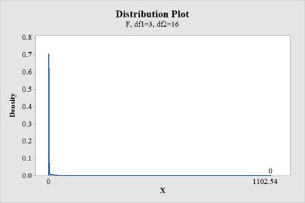
The enumerator degrees of freedom of F is 3 and the denominator degrees of freedom is 16.

P- value:

Software procedure:

Step by step procedure to obtain the P- value using the MINITAB software is given below:

• Choose Graph > Probability Distribution Plot choose View Probability > OK.
• From Distribution, choose ‘F’ distribution.
• Enter Numerator degree of freedom as 3.
• Enter Denominator degree of freedom as 16.
• Click the Shaded Area tab.
• Choose X value and Right tail for the region of the curve to shade.
• Enter the X value as 1,102.543.
• Click OK.

Output using the MINITAB software is given below:

Hence, the filled regression analysis table is,

Predictor	Coefficient		SE Coefficient	T		P
Constant	517.46		11.76	44.0017		0
$x_1$	11.4720		0.314	36.50		0
$x_2$	–8.1378		0.1969	–41.3296		0
$x_3$	10.8565		0.6652	16.3207		0
$S=10.2560$		$\underset{\_}{\text{R-Sq}=99.5\%}$			$\underset{\_}{\text{R-Sq}\left(\text{adj}\text{.}\right)=99.4\%}$
Analysis of Variance
Source	DF		SS	MS		F	P
Regression	3		347,300	115,767		1,102.543	0
Residual Error	16		1,683	105
Total	19		348,983

b.

To determine

Explain whether the model is significant at $\alpha =0.05$.

Also explain whether the model is significant at $\alpha =0.01$.

Answer to Problem 106SE

The test for the statistical significance of the regression at level of significance $\alpha =0.05$ and $\alpha =0.01$ suggest that there is sufficient evidence of statistical significance of the regression.

Explanation of Solution

Calculation:

Multiple regression model:

The regression model of the response variable y on k regressor variables, $X_1,X_2,\mathrm{...},X_k$ for n sets of observations, $\left(x_{i1},x_{i2},\mathrm{...},x_{ik},y_i\right)$ for $i=1,2,\mathrm{...},n$ is:

$Y={\beta }_0+{\beta }_1{x}_1+{\beta }_2{x}_2+\mathrm{...}+{\beta }_k{x}_k$.

Here, there are 3 regressors.

The model would be of the form:

$\widehat{y}={\beta }_0+{\beta }_1{x}_1+{\beta }_2{x}_2+{\beta }_3{x}_3$.

The parameter of the interest:

The parameters of the interest are the slope coefficients ${\beta }_1$ and ${\beta }_2$ corresponding to $x_1$  and $x_2$, respectively.

For level of significance$\alpha =0.05$:

Hypotheses:

Null hypothesis:

$H_0:{\beta }_1={\beta }_2={\beta }_3=0$.

That is, there is no statistical significance of the regression.

Alternative hypothesis:

$H_1:\text{At least one }{\beta }_i\text{ is non-zero}$, for $i=1,2,3$.

That is, there is statistical significance of the regression.

Level of significance:

Assume that, the level of significance is $\alpha =0.05$.

P-value:

From part (a), it is found that the P-value for the F-test of the regression is $\underset{\_}{P\text{-value}=0}$.

Decision rule:

If $P\text{-value}\le \alpha$, reject the null hypothesis $H_0$.

If,$P\text{-value}>\alpha$, fail to reject the null hypothesis $H_0$

Conclusion:

Here, the P-value is less than the level of significance.

That is, $P\text{-value}\left(=0\right)<\alpha \left(=0.05\right)$.

By rejection rule, reject the null hypothesis.

Hence, there is sufficient evidence of statistical significance of the regression.

For level of significance$\alpha =0.01$:

Hypotheses:

Null hypothesis:

$H_0:{\beta }_1={\beta }_2={\beta }_3=0$.

That is, there is no statistical significance of the regression.

Alternative hypothesis:

$H_1:\text{At least one }{\beta }_i\text{ is non-zero}$, for $i=1,2,3$.

That is, there is statistical significance of the regression.

Level of significance:

Assume that, the level of significance is $\alpha =0.01$.

P-value:

From part (a), it is found that the P-value for the F-test of the regression is $\underset{\_}{P\text{-value}=0}$.

Decision rule:

If $P\text{-value}\le \alpha$, reject the null hypothesis $H_0$.

If,$P\text{-value}>\alpha$, fail to reject the null hypothesis $H_0$

Conclusion:

Here, the P-value is less than the level of significance.

That is, $P\text{-value}\left(=0\right)<\alpha \left(=0.01\right)$.

By rejection rule, reject the null hypothesis.

Hence, there is sufficient evidence of statistical significance of the regression.

Conclusion:

Hence, there are enough evidence that there is statistical significance of at least one of the regressors for any of the given values $\alpha$.

c.

To determine

Explain about the contribution of the individual regressors to the model.

Answer to Problem 106SE

The tests for the statistical significance of the regressors at level of significance $\alpha =0.05$ suggest that there sufficient evidence of statistical significance of the coefficient of $x_1$, $x_2$ and $x_3$.

Explanation of Solution

Calculation:

Test for the statistical significance of $x_1$:

The parameter of the interest:

The parameter of the interest is the slope coefficient ${\beta }_1$ corresponding to $x_1$.

Hypotheses:

Null hypothesis:

$H_0:{\beta }_1=0$.

That is, there is no statistical significance of the coefficient of $x_1$.

Alternative hypothesis:

$H_1:{\beta }_1\ne 0$.

That is, there is statistical significance of the coefficient of $x_1$.

Level of significance:

Assume that level of significance is $\alpha =0.05$.

P-value:

From part (a), the P-value for the t-test of the coefficient of $x_1$ is $P\text{-value}=0$.

Decision rule:

If $P\text{-value}\le \alpha$, reject the null hypothesis $H_0$.

If,$P\text{-value}>\alpha$, fail to reject the null hypothesis $H_0$

Conclusion:

Here, the P-value is less than the level of significance.

That is, $P\text{-value}\left(=0\right)<\alpha \left(=0.05\right)$.

By rejection rule, reject the null hypothesis.

Hence, there is sufficient evidence of statistical significance of the coefficient of $x_1$.

Test for the statistical significance of $x_2$:

The parameter of the interest:

The parameter of the interest is the slope coefficient ${\beta }_2$ corresponding to $x_2$.

Hypotheses:

Null hypothesis:

$H_0:{\beta }_2=0$.

That is, there is no statistical significance of $x_2$.

Alternative hypothesis:

$H_1:{\beta }_2\ne 0$.

That is, there is statistical significance of the coefficient of $x_2$.

Level of significance:

Assume that, the level of significance is $\alpha =0.05$.

P-value:

From part (a), the P-value for the t-test of the coefficient of $x_2$ is $P\text{-value}=0$.

Decision rule:

If $P\text{-value}\le \alpha$, reject the null hypothesis $H_0$.

If,$P\text{-value}>\alpha$, fail to reject the null hypothesis $H_0$

Conclusion:

Here, the P-value is less than the level of significance.

That is, $P\text{-value}\left(=0\right)<\alpha \left(=0.05\right)$.

By rejection rule, reject the null hypothesis.

Hence, there is sufficient evidence of statistical significance of the coefficient of $x_2$.

Test for the statistical significance of $x_3$:

The parameter of the interest:

The parameter of the interest is the slope coefficient ${\beta }_2$ corresponding to $x_3$.

Hypotheses:

Null hypothesis:

$H_0:{\beta }_3=0$.

That is, there is no statistical significance of $x_3$.

Alternative hypothesis:

$H_1:{\beta }_3\ne 0$.

That is, there is statistical significance of the coefficient of $x_3$.

Level of significance:

Assume that, the level of significance is $\alpha =0.05$.

P-value:

From part (a), the P-value for the t-test of the coefficient of $x_3$ is $P\text{-value}=0$.

Decision rule:

If $P\text{-value}\le \alpha$, reject the null hypothesis $H_0$.

If,$P\text{-value}>\alpha$, fail to reject the null hypothesis $H_0$

Conclusion:

Here, the P-value is less than the level of significance.

That is, $P\text{-value}\left(=0\right)<\alpha \left(=0.05\right)$.

By rejection rule, reject the null hypothesis.

Hence, there is sufficient evidence of statistical significance of the coefficient of $x_3$.