
Concept explainers
Videos
The appraisal of a warehouse can appear straightforward compared to other appraisal assignments. A warehouse appraisal involves comparing a building that is primarily an open shell to other such buildings. However, there are still a number of warehouse attributes that are plausibly related to appraised value. The article “Challenges in Appraising ‘Simple’ Warehouse Properties” (Donald Sonneman, The Appraisal Journal, April 2001, 174–178) gives the accompanying data on truss height (ft), which determines how high stored goods can be stacked, and sale price ($) per square foot.
| Height | 12 | 14 | 14 | 15 | 15 | 16 | 18 | 22 | 22 | 24 |
| Price | 35.53 | 37.82 | 36.90 | 40.00 | 38.00 | 37.50 | 41.00 | 48.50 | 47.00 | 47.50 |
| Height | 24 | 26 | 26 | 27 | 28 | 30 | 30 | 33 | 36 |
| Price | 46.20 | 50.35 | 49.13 | 48.07 | 50.90 | 54.78 | 54.32 | 57.17 | 57.45 |
- a. Is it the case that truss height and sale price are “deter-ministically” related—i.e., that sale price is determined completely and uniquely by truss height? [Hint: Look at the data.]
- b. Construct a scatterplot of the data. What does it suggest?
- c. Determine the equation of the least squares line.
- d. Give a point prediction of price when truss height is 27 ft, and calculate the corresponding residual.
- e. What percentage of observed variation in sale price can be attributed to the approximate linear relationship between truss height and price?
a.
Explain whether the variable sale price is completely and uniquely determined by height.
Answer to Problem 68SE
No, the sale price is not uniquely determined by height.
Explanation of Solution
Given info:
The data represents the values of the variables height in feet and price in dollars of the stored goods.
Justification:
Uniquely determined:
Uniquely determined in the sense, for each value of the height, the sale price should be unique. That is, all the equal heights should be associated with same sale price and all the unequal heights should be associated with different sale price values.
From the dataset, it is observed that the equal heights also results in different sale price.
That is, the height value 14 is repeated twice with two different sale price values.
Hence, it can be concluded that sale price is not uniquely determined by height.
b.
Draw a scatterplot of the variables height and sale price.
Answer to Problem 68SE
Output using MINITAB software is given below:
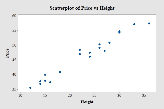
The association between the variables height and sale price is positive, strong and linear.
Explanation of Solution
Justification:
Software Procedure:
Step by step procedure to obtain scatterplot using Minitab software is given as,
- Choose Graph > Scatter plot.
- Choose Simple, and then click OK.
- Under Y variables, enter a column of Price.
- Under X variables, enter a column of Height.
- Click Ok.
Associated variables:
Two variables are associated or related if the value of one variable gives you information about the value of the other variable.
The two variables height and sale price are associated variables.
Direction of association:
If the increase in the values of one variable increases the values of another variable, then the direction is positive. If the increase in the values of one variable decreases the values of another variable, then the direction is negative.
Here, the value of sale price increases with the increase in the value of height.
Hence, the direction of the association is positive.
Form of the association between variable:
The form of the association describes whether the data points follow a linear pattern or some other complicated curves. For data if it appears that a line would do a reasonable job of summarizing the overall pattern in the data. Then, the association between two variables is linear.
From the scatterplot, it is observed that the pattern of the relationship between the variables height and sale price produces a relatively straight line.
Hence the form of the association between the variables height and sale price is linear.
Strength of the association:
The association is said to be strong if all the points are close to the straight line. It is said to be weak if all points are far away from the straight line and it is said to be moderate if the data points are moderately close to straight line.
From the scatterplot, it is observed that the variables will have perfect correlation between them.
Hence, the association between the variables is strong.
Observation:
From the scatterplot it is clear that, as the values of height increases the sale price of the stored goods also increases linearly. Thus, there is a positive association between the variables height and sale price.
c.
Find the regression line for the variables sale price
Answer to Problem 68SE
The regression line for the variables sale price
Explanation of Solution
Calculation:
Linear regression model:
In a linear regression model
Regression:
Software procedure:
Step by step procedure to obtain regression equation using MINITAB software is given as,
- Choose Stat > Regression > Fit Regression Line.
- In Response (Y), enter the column of Price.
- In Predictor (X), enter the column of Height.
- Click OK.
Output using MINITAB software is given below:
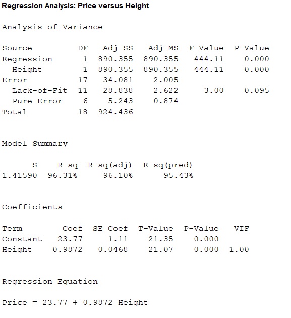
Thus, the regression line for the variables sale price
d.
Find the predicted value of sale price when the height is 27 feet.
Find the corresponding residual of the obtained point prediction.
Answer to Problem 68SE
The predicted value of sale price for 27 feet height stored goods is 50.4244.
The residual of the predicted value of sale price for 27 feet height stored goods is -2.3544.
Explanation of Solution
Calculation:
In a linear regression model
Here, the regression equation is
Point prediction of sale price when the height is 27 feet:
The predicted value of sale price for 27 ft height stored goods is obtained as follows:
Thus, the predicted value of sale price for 27 ft height stored goods is 50.4244.
Residual:
The residual is defined as
If the observed value is less than predicted value then the residual will be negative and if the observed value is greater than predicted value then the residual will be positive.
Residual of predicted value of sale price when the height is 27ft:
The predicted value of sale price for 27 feet height stored goods is 50.4244.
From the given data, the observed value of sale price corresponding to height 27ft is 48.07.
The general formula to obtain residuals is,
Here, the residual values are obtained as follows:
Thus, for a height of 27, the observed sale price is 48.07 and the predicted sale price is 50.4244.
Therefore, the residual is,
Hence, the residual is negative and the predicted sale price 50.4244 is higher than the actual sale price for a height of 27 ft.
Hence, it is preferable to have negative residual.
e.
Find the proportion of observed variation in sale price that can be explained by the obtained regression model.
Answer to Problem 68SE
The proportion of observed variation in sale price that can be explained by the obtained regression model is 96.31%.
Explanation of Solution
Justification:
The coefficient of determination (
The general formula to obtain coefficient of variation is,
From the regression output obtained in part (a), the value of coefficient of determination is 0.631.
Thus, the coefficient of determination is
The coefficient of determination describes the amount of variation in the observed values of the response variable that is explained by the regression.
Interpretation:
From this coefficient of determination it can be said that, the height can explain only 96.31% variability in sale price. Then remaining variability of sale price is explained by other variables.
Thus, the percentage of variation in the observed values of sale price that is explained by the regression is 96.31%, which indicates that 96.31% of the variability in sale price is explained by variability in the height using the linear regression model.
Want to see more full solutions like this?
Chapter 12 Solutions
Probability and Statistics for Engineering and the Sciences


 Glencoe Algebra 1, Student Edition, 9780079039897...AlgebraISBN:9780079039897Author:CarterPublisher:McGraw Hill
 Big Ideas Math A Bridge To Success Algebra 1: Stu...AlgebraISBN:9781680331141Author:HOUGHTON MIFFLIN HARCOURTPublisher:Houghton Mifflin Harcourt
 College Algebra (MindTap Course List)AlgebraISBN:9781305652231Author:R. David Gustafson, Jeff HughesPublisher:Cengage Learning
 Holt Mcdougal Larson Pre-algebra: Student Edition...AlgebraISBN:9780547587776Author:HOLT MCDOUGALPublisher:HOLT MCDOUGAL