
Concept explainers
Videos
a.
Check whether a linear model is appropriate for the data using the
a.
Answer to Problem 48E
Output using MINITAB software is given below:
Yes, a simple linear model is appropriate for the data.
Explanation of Solution
Given info:
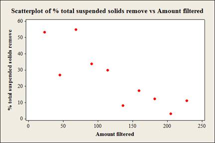
The data represents the values of the variables % total suspended solids removed
Justification:
Software Procedure:
Step by step procedure to obtain scatterplot using MINITAB software is given as,
- Choose Graph > Scatter plot.
- Choose Simple, and then click OK.
- Under Y variables, enter a column of % Total suspended solids removed.
- Under X variables, enter a column of Amount filtered.
- Click Ok.
Observation:
From the scatterplot it is clear that, as the values of amount filtered increases the values of % total suspended solids removed decreases linearly. Thus, there is a negative association between the variables amount filtered and % total suspended solids removed.
Appropriateness of regression linear model:
The conditions for a scatterplot that is well fitted for the data are,
- Straight Enough Condition: The relationship between y and x straight enough to proceed with a linear regression model.
- Outlier Condition: No outlier must be there which influences the fit of the least square line.
- Thickness Condition: The spread of the data around the generally straight relationship seem to be consistent for all values of x.
The scatterplot shows a fair enough linear relationship between the variables amount filtered and % total suspended solids removed. The spread of the data seem to roughly consistent.
Moreover, the scatterplot does not show any outliers.
Therefore, all the three conditions of appropriateness of simple linear model are satisfied.
Thus, a linear model is appropriate for the data.
b.
Find the regression line for the variables % total suspended solids removed
b.
Answer to Problem 48E
The regression line for the variables % total suspended solids removed
Explanation of Solution
Calculation:
Linear regression model:
A linear regression model is given as
A linear regression model is given as
In the given problem the % of total suspended solids remove is the response variable y and the amount filtered is the predictor variable x
Regression:
Software procedure:
Step by step procedure to obtain regression equation using MINITAB software is given as,
- Choose Stat > Regression > Fit Regression Line.
- In Response (Y), enter the column of Removal efficiency.
- In Predictor (X), enter the column of Inlet temperature.
- Click OK.
The output using MINITAB software is given as,
Thus, the regression line for the variables % total suspended solids removed
Interpretation:
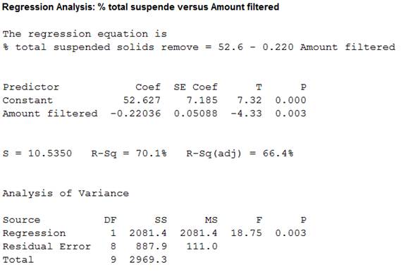
The slope estimate implies a decrease in % total suspended solids removed by 22.0% for every 1,000 liters increase in amount filtered. It can also be said that, for every 1% increase in amount filtered the % total suspended solids removed decreases 22%.
c.
Find the proportion of observed variation in % total suspended solids removed that can be explained by amount filtered using the simple linear regression model.
c.
Answer to Problem 48E
The proportion of observed variation in % total suspended solids removed that can be explained by amount filtered using the simple linear regression model is
Explanation of Solution
Justification:
The coefficient of determination (
The general formula to obtain coefficient of variation is,
From the regression output obtained in part (b), the value of coefficient of determination is 0.701.
Thus, the coefficient of determination is
Interpretation:
From this coefficient of determination it can be said that, the amount filtered can explain only 70.1% variability in % total suspended solids removed. Then remaining variability of % total suspended solids removed is explained by other variables.
Thus, the percentage of variation in the observed values of %total suspended solids removed that is explained by the regression is 70.1%, which indicates that 70.1% of the variability in %total suspended solids removed is explained by variability in the amount filtered using the linear regression model.
d.
Test whether there is enough evidence to conclude that the predictor variable amount filtered is useful for predicting the value of the response variable %total suspended solids removed at
d.
Answer to Problem 48E
There is sufficient evidence to conclude that the predictor variable amount filtered is useful for predicting the value of the response variable %total suspended solids removed.
Explanation of Solution
Calculation:
From the MINITAB output obtained in part (b), the regression line for the variables %total suspended solids removed
The test hypotheses are given below:
Null hypothesis:
That is, there is no useful relationship between the variables %total suspended solids removed
Alternative hypothesis:
That is, there is useful relationship between the variables %total suspended solids removed
T-test statistic:
The test statistic is,
From the MINITAB output obtained in part (b), the test statistic is -4.33 and the P-value is 0.003.
Thus, the value of test statistic is -4.33 and P-value is 0.003.
Level of significance:
Here, level of significance is
Decision rule based on p-value:
If
If
Conclusion:
The P-value is 0.003 and
Here, P-value is less than the
That is
By the rejection rule, reject the null hypothesis.
Thus, there is sufficient evidence to conclude that the predictor variable amount filtered is useful for predicting the value of the response variable %total suspended solids removed.
e.
Test whether there is enough evidence to infer that the true average decrease in “%total suspended solids removed” associated with 10,000 liters increase in “amount filtered” is greater than or equal to 2 at
e.
Answer to Problem 48E
There is no sufficient evidence to infer that the true average decrease in “%total suspended solids removed” associated with 10,000 liters increase in “amount filtered” is greater than or equal to 2.
Explanation of Solution
Calculation:
Linear regression model:
A linear regression model is given as
A linear regression model is given as
From the MINITAB output in part (b), the slope coefficient of the regression equation is
Here,
Here, the claim is that, when the amount filtered is increased from 10,000 liters the true average decrease in %total suspended solids removed is greater than or equal to 2.
The claim states that, amount filtered is increased by 10,000 liters.
Decrease in the %total suspended solids removed for 1,000 liters increase in amount filtered:
The true average decrease in the %total suspended solids removed for 1,000 liters increase in amount filtered is,
That is, when the amount filtered is increased by 1,000 liters the true average decrease in %total suspended solids removed is greater than or equal to 0.2.
The test hypotheses are given below:
Null hypothesis:
That is, the true average decrease in %total suspended solids removed is greater than or equal to 0.2.
Alternative hypothesis:
That is, the true average decrease in %total suspended solids removed is less than 0.2.
Test statistic:
The test statistic is,
Degrees of freedom:
The sample size is
The degrees of freedom is,
Thus, the degree of freedom is 8.
Here, level of significance is
Critical value:
Software procedure:
Step by step procedure to obtain the critical value using the MINITAB software:
- Choose Graph > Probability Distribution Plot choose View Probability > OK.
- From Distribution, choose ‘t’ distribution and enter 8 as degrees of freedom.
- Click the Shaded Area tab.
- Choose Probability Value and Left Tail for the region of the curve to shade.
- Enter the Probability value as 0.05.
- Click OK.
Output using the MINITAB software is given below:
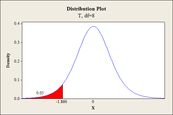
From the output, the critical value is –1.860.
Thus, the critical value is
From the MINITAB output obtained in part (b), the estimate of error standard deviation of slope coefficient is
Test statistic under null hypothesis:
Under the null hypothesis, the test statistic is obtained as follows:
Thus, the test statistic is -0.3931.
Decision criteria for the classical approach:
If
Conclusion:
Here, the test statistic is -0.3931 and critical value is –1.860.
The t statistic is less than the critical value.
That is,
Based on the decision rule, reject the null hypothesis.
Hence, the true average decrease in %total suspended solids removed is not greater than or equal to 0.2.
Therefore, there is no sufficient evidence to infer that the true average decrease in “%total suspended solids removed” associated with 10,000 liters increase in “amount filtered” is greater than or equal to 2.
f.
Find the 95% specified confidence interval for the true
Compare the width of the confidence intervals for 100,000 liters and 200,000 liters amount filtered.
f.
Answer to Problem 48E
The 95% specified confidence interval for the true mean %total suspended solids removed when the amount filtered is 100,000 liters is
The confidence interval for 100,000 liters of amount filtered will be narrower than the interval for 200,000 liters of amount filtered.
Explanation of Solution
Calculation:
From the MINITAB output obtained in part (b), the regression line for the variables %total suspended solids removed
Here, the variable amount filtered
Hence, the value of 100,000 for amount filtered is
Expected %total suspended solids removed when the amount filtered is
The expected value of %total suspended solids removed with
Thus, the expected value of %total suspended solids removed with
Confidence interval:
The general formula for the
Where,
From the MINITAB output in part (a), the value of the standard error of the estimate is
The value of
From the give data, the sum of amount filtered is
The mean amount filtered is,
Thus, the mean amount filtered is
Covariance term
The value of
Thus, the covariance term
Critical value:
For 95% confidence level,
Degrees of freedom:
The sample size is
The degrees of freedom is,
From Table A.5 of the t-distribution in Appendix A, the critical value corresponding to the right tail area 0.025 and 8 degrees of freedom is 2.306.
Thus, the critical value is
The 95% confidence interval is,
Thus, the 95% specified confidence interval for the true mean %total suspended solids removed when the amount filtered is 100,000 liters is
Interpretation:
There is 95% confident that, the true mean %total suspended solids removed when the amount filtered is 100,000 liters lies between 22.37244 and 38.82756.
Comparison:
For 100,000 amount filtered, the value of x is
The mean amount filtered is
Here, the observation
The general formula to obtain
For
For
In the two quantities, the only difference is the values
In general, the value of the quantity
Therefore, the value
The confidence interval will be wider for large value of
Here,
Thus, the confidence interval is wider for
g.
Find the 95% prediction interval for the single value of %total suspended solids removed when the amount filtered is 100,000 liters.
Compare the width of the prediction intervals for 100,000 liters and 200,000 liters amount filtered.
g.
Answer to Problem 48E
The 95% prediction interval for the single value of %total suspended solids removed when the amount filtered is 100,000 liters is
The prediction interval for 100,000 liters of amount filtered will be narrower than the interval for 200,000 liters of amount filtered.
Explanation of Solution
Calculation:
From the MINITAB output obtained in part (b), the regression line for the variables %total suspended solids removed
From part (c), the
Prediction interval for a single future value:
Prediction interval is used to predict a single value of the focus variable that is to be observed at some future time. In other words it can be said that the prediction interval gives a single future value rather than estimating the mean value of the variable.
The general formula for
where
From the MINITAB output in part (b), the value of the standard error of the estimate is
From part (c), the mean chlorine flow is
Critical value:
For 95% confidence level,
Degrees of freedom:
The sample size is
The degrees of freedom is,
From Table A.5 of the t-distribution in Appendix A, the critical value corresponding to the right tail area 0.025 and 8 degrees of freedom is 2.306.
Thus, the critical value is
The 95% prediction interval is,
Thus, the 95% prediction interval for the single value of %total suspended solids removed when the amount filtered is 100,000 liters is
Interpretation:
For repeated samples, there is 95% confident that the single value of % total suspended solids removed when the amount filtered is 100,000 liters will lie between 4.950886 and 56.24911.
Comparison:
For 100,000 amount filtered, the value of x is
The mean amount filtered is
Here, the observation
The general formula to obtain
For
For
In the two quantities, the only difference is the values
In general, the value of the quantity
Therefore, the value
The prediction interval will be wider for large value of
Here,
Thus, the prediction interval is wider for
Want to see more full solutions like this?
Chapter 12 Solutions
Probability and Statistics for Engineering and the Sciences


- Lactation promotes a temporary loss of bone mass to provide adequate amounts of calcium for milk production. The paper “Bone Mass Is Recovered from Lactation to Postweaning in Adolescent Mothers with Low Calcium Intakes” (Amer. J. of Clinical Nutr., 2004: 1322–1326) gave the following data on total body bone mineral content (TBBMC) (g) for a sample both during lactation (L) and in the postweaning period (P). SubjectL 1928 2549 2825 1924 1628 2175 2114 2621 1843 2541P 2126 2885 2895 1942 1750 2184 2164 2626 2006 2627 Does the data suggest that true average total body bone mineral content during postweaning exceeds that during lactation by more than 25 g? State and test the appropriate hypotheses using a significance level of .05.arrow_forwardThe article “Effects of Diets with Whole Plant-Origin Proteins Added with Different Ratiosof Taurine:Methionine on the Growth, Macrophage Activity and Antioxidant Capacity ofRainbow Trout (Oncorhynchus mykiss) Fingerlings” (O. Hernandez, L. Hernandez, et al.,Veterinary and Animal Science, 2017:4-9) reports that a sample of 210 juvenile rainbowtrout fed a diet fortified with equal amounts of the amino acids taurine and methionine for aperiod of 70 days had a mean weight gain of 313 percent with a standard deviation of 25, while 210 fish fed with a control diet had a mean weight gain of 233 percent with a standard deviation of 19. Units are percent. Find a 99% confidence interval for the difference in weight gain on the two diets.arrow_forwardThe article “Hydrogeochemical Characteristics of Groundwater in a Mid-Western CoastalAquifer System” (S. Jeen, J. Kim, et al., Geosciences Journal, 2001:339–348) presentsmeasurements of various properties of shallow groundwater in a certain aquifer system inKorea. Following are measurements of electrical conductivity (in microsiemens percentimeter) for 23 water samples.2099 528 2030 1350 1018 384 14991265 375 424 789 810 522 513488 200 215 486 257 557 260461 500Find the mean.Find the standard deviation.Find the median.Construct a dotplot.Find the 10% trimmed mean.Find the first quartile.Find the third quartile.Find the interquartile range.Construct a boxplot.Which of the points, if any, are outliers?If a histogram were constructed, would it be skewed to the left, skewed to the right, orapproximately symmetric?arrow_forward
- Stressed-Out Bus Drivers. Previous studies have shown that urban bus drivers have an extremely stressful job, and a large proportion of drivers retire prematurely with disabilities due to occupational stress. In the paper, “Hassles on the Job: A Study of a Job Intervention With Urban Bus Drivers” (Journal of Organizational Behavior, Vol. 20, pp. 199–208), G. Evans et al. examined the effects of an intervention program to improve the conditions of urban bus drivers.Amongother variables, the researchers monitored diastolic blood pressure of bus drivers in downtown Stockholm, Sweden. The data, in millimeters of mercury (mm Hg), on the WeissStats site are based on the blood pressures obtained prior to intervention for the 41 bus drivers in the study. Use the technology of your choice to do the following. a. Obtain a normal probability plot, boxplot, histogram, and stemand-leaf diagram of the data. b. Based on your results from part (a), can you reasonably apply the one-mean t-test to the…arrow_forwardSuppose a researcher is interested inthe effectiveness in a new childhood exercise program implemented in a SRS of schools across a particular county. In order to test the hypothesis that the new program decreases BMI (Kg/m2), the researcher takes a SRS of children from schools where the program is employed and a SRS from schools that do not employ the program and compares the results. Assume the following table represents the SRSs of students and their BMIs. Student intervention group BMI (kg/m2) Student control group BMI (kg/m2) A 18.6 A 21.6 B 18.2 B 18.9 C 19.5 C 19.4 D 18.9 D 22.6 E 24.1 F 23.6 A) Assuming that all the necessary conditions are met (normality, independence, etc.) carry out the appropriate statistical test to determine if the new exercise program is effective. Use an alpha level of 0.05. Do not assume equal variances.B) Construct a 95% confidence interval about your estimate for the average difference in BMI between the groups.arrow_forwardAn article in the Journal of the Electrochemical Society (Vol. 139, No. 2, 1992, pp. 524–532) describes anexperiment to investigate the low-pressure vapor deposition of polysilicon. The experiment was carried outin a large-capacity reactor at Sematech in Austin, Texas. The reactor has several wafer positions, and fourof these positions are selected at random. The response variable is film thickness uniformity. Threereplicates of the experiment were run, and the data are as follows:a. Test the significance of these wafer position with α=0.05.b. If proven significant, perform a multiple comparison method using Fisher’s LSD.arrow_forward
- Following are the protein contents measured in two types of species:Species 1: 0.72 1.12 0.81 0.89 0.72 0.81 1.01 0.75 0.83Species 2: 1.21 0.93 0.80 1.12 1.22 0.94 0.87 i) Assuming normality, test the hypothesis that the two species have the sameaverage protein contents by using 5-step hypothesis testing procedure at 5 %level of significance, and using the critical values approach.ii) Calculate the p-value of this test and make decision.iii) Write down the standard error of this test and calculate its numerical value ?arrow_forwardThe table below shows the numbers of bushels of barley cultivated per acre for 12 one-acre plots of land for two different strains of barley, PHT-34 and CBX-21. PHT-34 CBX-21 43 55 49 46 47 43 38 44 47 45 45 49 50 47 46 59 46 52 46 49 45 48 43 51 Determine the minimum data value, the quartiles, and the maximum data value for the PHT-34 and CBX-21 data sets. PHT-34 CBX-21 min Q1 Q2 Q3 maxarrow_forwardThe dry shear strength of birch plywood bonded with different resin glues was studied with a completely randomized designed experiment. Here are the data: Glue A (102; 58; 45; 79; 68; 63; 117) Glue C (100; 102; 80; 119) Glue F (220; 243; 189; 176; 176). What is the F critical value at the 2.5% significance levelarrow_forward
- An article in Knee Surgery, Sports Traumatology, Arthroscopy (2005, Vol. 13, pp. 273-279) considered arthroscopic meniscal repair with an absorbable screw. Results showed that for tears greater than 25 millimeters, 14 of 18 (78%) repairs were successful, but for shorter tears, 22 of 30 (73%) repairs were successful. A doctor would like to know if there is evidence that the success rate is greater for longer tears. The P-value for the test H0: p1 = p2 versus H1: p1 > p2 is closest to:arrow_forwardAn article in the Journal of Quality Technology (Vol. 13, No. 2, 1981, pp. 111–114) describes an experimentthat investigates the effects of four bleaching chemicals on pulp brightness. These four chemicals wereselected at random from a large population of potential bleaching agents. The data are as follows:a. Test the significance of these chemical types with α=0.05.b. If proven significant, perform a multiple comparison method using Fisher’s LSDarrow_forwardWhen determining whether grounding accidents and hull failures result in different spillage (is there a difference between spills caused by grounding or hull failures) would I use a two tail t test to decide this?arrow_forward
 MATLAB: An Introduction with ApplicationsStatisticsISBN:9781119256830Author:Amos GilatPublisher:John Wiley & Sons Inc
 Probability and Statistics for Engineering and th...StatisticsISBN:9781305251809Author:Jay L. DevorePublisher:Cengage Learning
 Statistics for The Behavioral Sciences (MindTap C...StatisticsISBN:9781305504912Author:Frederick J Gravetter, Larry B. WallnauPublisher:Cengage Learning
 Elementary Statistics: Picturing the World (7th E...StatisticsISBN:9780134683416Author:Ron Larson, Betsy FarberPublisher:PEARSON
 The Basic Practice of StatisticsStatisticsISBN:9781319042578Author:David S. Moore, William I. Notz, Michael A. FlignerPublisher:W. H. Freeman
 Introduction to the Practice of StatisticsStatisticsISBN:9781319013387Author:David S. Moore, George P. McCabe, Bruce A. CraigPublisher:W. H. Freeman