
Concept explainers
Videos
The North Valley Real Estate data reports information on homes on the market.
- a. Let selling price be the dependent variable and size of the home the independent variable. Determine the regression equation. Estimate the selling price for a home with an area of 2,200 square feet. Determine the 95% confidence interval for all 2,200 square foot homes and the 95% prediction interval for the selling price of a home with 2,200 square feet.
- b. Let days-on-the-market be the dependent variable and price be the independent variable. Determine the regression equation. Estimate the days-on-the-market of a home that is priced at $300,000. Determine the 95% confidence interval of days-on-the-market for homes with a mean price of $300,000, and the 95% prediction interval of days-on-the-market for a home priced at $300,000.
- c. Can you conclude that the independent variables “days on the market” and “selling price” are
positively correlated ? Are the size of the home and the selling price positively correlated? Use the .05 significance level. Report the p-value of the test. Summarize your results in a brief report.
a.
Find the regression equation.
Find the selling price of a home with an area of 2,200 square feet.
Construct a 95% confidence interval for all 2,200 square foot homes.
Construct a 95% prediction interval for the selling price of a home with 2,200 square feet.
Answer to Problem 62DA
The regression equation is
The selling price of a home with an area of 2,200 square feet is 222,624.423.
The 95% confidence interval for all 2,200 square foot homes is
The 95% prediction interval for the selling price of a home with 2,200 square feet is
Explanation of Solution
Here, the selling price is the dependent variable and size of the home is the independent variable.
Step-by-step procedure to obtain the ‘regression equation’ using MegaStat software:
- In an EXCEL sheet enter the data values of x and y.
- Go to Add-Ins > MegaStat > Correlation/Regression > Regression Analysis.
- Select input range as ‘Sheet1!$B$2:$B$106’ under Y/Dependent variable.
- Select input range ‘Sheet1!$A$2:$A$106’ under X/Independent variables.
- Select ‘Type in predictor values’.
- Enter 2,200 as ‘predictor values’ and 95% as ‘confidence level’.
- Click on OK.
Output obtained using MegaStat software is given below:
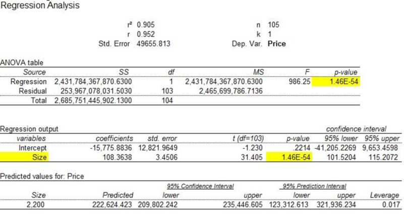
From the regression output, it is clear that
The regression equation is
The selling price of a home with an area of 2,200 square feet is 222,624.423.
The 95% confidence interval for all 2,200 square foot homes is
The 95% prediction interval for the selling price of a home with 2,200 square feet is
b.
Find the regression equation.
Find day-on-the-market for homes with a mean price at $300,000.
Construct a 95% confidence interval of day-on-the-market for homes with a mean price at $300,000.
Construct a 95% prediction interval day-on-the-market for a home priced at $300,000.
Answer to Problem 62DA
The regression equation is
The day-on-the-market for homes with a mean price at $300,000 is 28.930.
The 95% confidence interval of day-on-the-market for homes with a mean price at $300,000 is
The 95% prediction interval day-on-the-market for a home priced at $300,000 is
Explanation of Solution
Here, the selling price is the dependent variable and size of the home is the independent variable.
Step-by-step procedure to obtain the ‘regression equation’ using MegaStat software:
- In an EXCEL sheet enter the data values of x and y.
- Go to Add-Ins > MegaStat > Correlation/Regression > Regression Analysis.
- Select input range as ‘Sheet1!$C$2:$C$106’ under Y/Dependent variable.
- Select input range ‘Sheet1!$B$2:$B$106’ under X/Independent variables.
- Select ‘Type in predictor values’.
- Enter 300,000 as ‘predictor values’ and 95% as ‘confidence level’.
- Click on OK.
Output obtained using MegaStat software is given below:
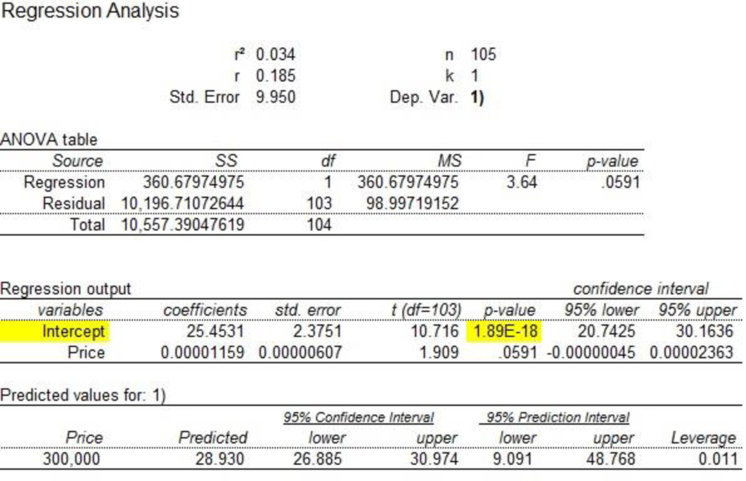
From the regression output, it is clear that
The regression equation is
The day-on-the-market for homes with a mean price at $300,000 is 28.930.
The 95% confidence interval of day-on-the-market for homes with a mean price at $300,000 is
The 95% prediction interval day-on-the-market for a home priced at $300,000 is
c.
Check whether the independent variables “day on the market” and “selling price” are positively correlated.
Check whether the independent variables “selling price” and “size of the home” are positively correlated.
Report the p-value of the test and summarize the result.
Answer to Problem 62DA
There is a positive association between “day on the market” and “selling price”.
There is a positive association between “selling price” and “size of the home”.
Explanation of Solution
Denote the population correlation as
Check the correlation between independent variables “day on the market” and “selling price” is positive
The hypotheses are given below:
Null hypothesis:
That is, the correlation between “day on the market” and “selling price” is less than or equal to zero.
Alternative hypothesis:
That is, the correlation between “day on the market” and “selling price” is positive.
Test statistic:
The test statistic is as follows:
Here, the sample size is 105 and the correlation coefficient is 0.185.
The test statistic is as follows:
The degrees of freedom is as follows:
The level of significance is 0.05. Therefore,
Critical value:
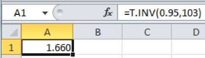
Step-by-step software procedure to obtain the critical value using EXCEL software:
- Open an EXCEL file.
- In cell A1, enter the formula “=T.INV (0.95, 103)”.
Output obtained using EXCEL is given as follows:
Decision rule:
Reject the null hypothesis H0, if
Conclusion:
The value of test statistic is 1.91 and the critical value is 1.660.
Here,
By the rejection rule, reject the null hypothesis.
Thus, there is enough evidence to infer that there is a positive association between “day on the market” and “selling price”.
The p-value of the test is 0.0591.
Check the correlation between independent variables “size of the home” and “selling price” is positive:
The hypotheses are given below:
Null hypothesis:
That is, the correlation between “size of the home” and “selling price” is less than or equal to zero.
Alternative hypothesis:
That is, the correlation between “size of the home” and “selling price” is positive.
Test statistic:
The test statistic is as follows:
Here, the sample size is 105 and the correlation coefficient is 0.952.
The test statistic is as follows:
Decision rule:
Reject the null hypothesis H0, if
Conclusion:
The value of test statistic is 31.56 and the critical value is 1.660.
Here,
By the rejection rule, reject the null hypothesis.
Thus, there is enough evidence to infer that there is a positive association between “size of the home” and “selling price”.
The p-value is approximately 0.
Want to see more full solutions like this?
Chapter 13 Solutions
EBK STATISTICAL TECHNIQUES IN BUSINESS


- Which of the following is a correct explanation of the confidence interval for the regression slope? Choose the BEST option. Group of answer choices The Tip is expected to increase by between $32.389 and $81.525 for every dollar increase in Sale amount. The average Sale amount is expected to decrease by between $0.080 and $0.174 for every dollar increase in Tip. The Tip is expected to decrease by between $0.080 and $0.174 for every dollar increase in Sale amount. The average Tip is expected to increase by between $32.389 and $81.525 for every dollar increase in Sale amount. The average Tip is expected to increase by between $0.080 and $0.174 for every dollar increase in Sale amount. The average Sale amount is expected to increase by between $32.389 and $81.525 for every dollar increase in Tip.arrow_forwardThe sample observation below were randomly selected. (a) Determine the regression equation, (b) Determine the expected value of Y if X=9, (c) Determine the 0.90 confidence interval for the mean predicted when X=9, and (d) Determine the 0.90 prediction interval for an individual predicted when X=9. x 4,5,3,6,10 y 4 6 5 7 7arrow_forwardThe final exam score was recorded for each Harper statistics student in a sample of 30. A 95% confidence interval forarrow_forward
- Consider the following set of dependent and independent variables. Use these data to complete parts a and b below. y 48 46 42 42 35 32 30 25 16 x1 78 66 80 52 42 46 30 15 13 x2 22 26 21 20 14 16 9 13 11 a) Construct a 95% confidence interval for the regression coefficient for x1 and interpret its meaning. -The 95% confidence interval for the true population coefficient B1 is ____ to ____. b) Construct a 99% confidence interval for the regression coefficient for x2 and interpret its meaning. -The 99% confidence interval for the true population coefficient B2 is approximately from ___ to ___. I have many of these questions, i need help knowing what steps to take! Thanks!arrow_forwardIn a situation where the sample size was decreased from 39 to 29 in a normally distributed data set, what would be the impact on the confidence interval?arrow_forwardRefer to 9.3.4 below and Let X = 1.6 and construct the 95 percent confidence interval for μy|x and construct the 95 percent prediction interval for Y. 9.3.4 Reiss et al. (A-3) compared point-of-care and standard hospital laboratory assays for monitoring patients receiving a single anticoagulant or a regimen consisting of a combination of anticoagulants. It is quite common when comparing two measuring techniques, to use regression analysis in which one variable is used to predict another. In the present study, the researchers obtained measures of international normalized ratio (INR) by assay of capillary and venous blood samples collected from 90 subjects taking warfarin. INR, used especially when patients are receiving warfarin, measures the clotting ability of the blood. Point-of-care testing for INR was conducted with the CoaguChek assay product. Hospital testing was done with standard hospital laboratory assays. The authors used the hospital assay INR level to predict the CoaguChek…arrow_forward
- The following table lists the monthly incomes (in hundreds of dollars) and the monthly rents paid (in hundreds of dollars) by a sample of six families. Monthly Income Monthly Rent 24 7.0 16 4.5 19 6.5 31 11.6 10 4.5 27 8.5 1.The 99% confidence interval for the slope, B, of the population regression line is (2 decimals): __________________________________________ 2. The null hypothesis is that the slope of the population regression line of monthly rent on monthly income is zero and the alternative hypothesis is that the slope of this population regression line is greater than zero. The significance level is 1%. What is the critical value of t (3 decimals)? __________________________________________ 3. The null hypothesis is that the slope of the population regression line of monthly rent on monthly income is zero and the alternative hypothesis is that the slope of this population regression line is greater than zero. The significance level is 1%. What is…arrow_forwardA medical researcher treats 400 subjects with high cholesterol using a new drug. After two months of taking the drug, the average decrease in cholesterol level is = 90 and the researcher assumes that the decrease in cholesterol follows a Normal distribution, with unknown mean and standard deviation = 20. A 95% confidence interval for is: a. 90 ± 2.94. b. 90 ± 2.35. c. 90 ± 1.96. d. 90 ± 3.92arrow_forwardSarah is the office manager for a group of financial advisors who provide financial services forindividual clients. She would like to investigate whether a relationship exists between the numberof presentations made to prospective clients in a month and the number of new clients per month.The following table shows the number of presentations and corresponding new clients for aa random sample of six employees.Employee Presentations New Clients1 7 22 9 33 9 44 10 35 11 56 12 3Sarah would like to use simple regression analysis to estimate the number of new clients permonth based on the number of presentations made by the employee per month. The test statisticfor testing the hypothesis that the population coefficient of determination is greater than zero is________. A) 1.03 B) 1.45 C) -1.16 D) 0.35arrow_forward
- In order to determine a realistic price for a new product that a company wants to market the company’s research department selected 10 sites thought to have essentially identical sales potential and offered the product in each at a different price. The resulting sales are recorded in the accompanying table: Price ($) Sales ($1,000s) 15.00 15 15.50 14 16.00 16 16.50 9 17.00 12 17.50 10 18.00 8 18.50 9 19.00 6 19.50 5 c). Find the equation of the sample regression line using Minitab. d). Interpret the meaning of the coefficients of the equation of the sample regression line.arrow_forwardA U.S. Food Survey showed that Americans routinely eat beef in their diet. Suppose that in a study of 49 consumers in Illinois and 64 consumers in Texas the following results were obtained from two samples regarding average yearly beef consumption: Illinois Texas = 49 = 64 = 54.1lb = 60.4lb S1 = 7.0 S2 = 8.0 Develop a 95% confidence Interval Estimate for the difference between the two population means.arrow_forwardIn Exercises, presume that the assumptions for regression inferences are met.Crown-Rump Length. Following are the data on age of fetuses and length of crown-rump from Exercise. x 10 10 13 13 18 19 19 23 25 28 y 66 66 108 106 161 166 177 228 235 280 a. Determine a point estimate for the mean crown-rump length of all 19-week-old fetuses.b. Find a 90% confidence interval for the mean crown-rump length of all 19-week-old fetuses.c. Find the predicted crown-rump length of a 19-week-old fetus.d. Determine a 90% prediction interval for the crown-rump length of a 19-week-old fetus.ExerciseApplying the Concepts and SkillsIn Exercises, we repeat the information from Exercises. For each exercise here, discuss what satisfying Assumptions 1–3 for regression inferences by the variables under consideration would mean.arrow_forward
 Glencoe Algebra 1, Student Edition, 9780079039897...AlgebraISBN:9780079039897Author:CarterPublisher:McGraw Hill