
Videos
The following data resulted from an experiment to assess the potential of unburnt colliery spoil as a medium for plant growth. The variables are x 5 acid extractable cations and y 5 exchangeable acidity/total cation exchange capacity (“Exchangeable Acidity in Unburnt Colliery Spoil,” Nature, 1969: 161):
| x | -5 | 16 | 26 | 30 | 38 | 52 | |
| y | 1.50 | 1.46 | 1.32 | 1.17 | .96 | .78 | .77 |
| x | 58 | 67 | 81 | 96 | 100 | 113 | |
| y | .91 | .78 | .69 | .52 | .48 | .55 |
Standardizing the independent variable x to obtain
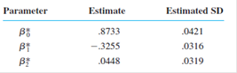
a. Estimate
b. Compute the value of the coefficient of multiple determination. (See Exercise 28(c).)
c. What is the estimated regression function
d. What is the estimated standard deviation of
e. Carry out a test using the standardized estimates to decide whether the quadratic term should be retained in the model. Repeat using the unstandardized estimates. Do your conclusions differ?
Want to see the full answer?
Check out a sample textbook solution
Chapter 13 Solutions
Probability and Statistics for Engineering and the Sciences


- The following fictitious table shows kryptonite price, in dollar per gram, t years after 2006. t= Years since 2006 0 1 2 3 4 5 6 7 8 9 10 K= Price 56 51 50 55 58 52 45 43 44 48 51 Make a quartic model of these data. Round the regression parameters to two decimal places.arrow_forwardBased on the data shown below, a statistician calculates a linear model y=2.41x+2.76y=2.41x+2.76. x y 4 12.5 5 14.35 6 16.9 7 20.65 8 22.1 9 23.95 Use the model to estimate the yy-value when x=9x=9y=y=arrow_forwardConsider the following two a.m. peak work trip generation models, estimated by household linear regression: T = 0.62 + 3.1 X1 + 1.4 X2 R2= 0.590 (2.3) (7.1) (5.9) T = 0.01 + 2.4 X1 + 1.2 Z1 + 4.0 Z2 R2= 0.598 (0.8) (4.2) (1.7) (3.1) X1 = number of workers in the household X2 = number of cars in the household, Z1 is a dummy variable which takes the value 1 if the household has one car, Z2 is a dummy variable which takes the value 1 if the household has two or more cars. Compare the two models and choose the best. If a zone has 1000 households, of which 50% have no car, 35% have one car, and the rest have exactly two cars, estimate the total number of trips generated by this zone. Use the preferred trip generation model and assume that each household has an average of two workersarrow_forward
- An article in the Journal of Applied Polymer Science (Vol. 56, pp. 471–476, 1995) studied the effect of the mole ratio of sebacic acid on the intrinsic viscosity of copolyesters.- The data follows: Viscosity 0.45 0.2 0.34 0.58 0.7 0.57 0.55 0.44 Mole ratio 1 0.9 0.8 0.7 0.6 0.5 0.4 0.3 (a) Construct a scatter diagram of the data.arrow_forwardThe following are data on the average weekly profits(in $1,000) of five restaurants, their seating capacities, andthe average daily traffic (in thousands of cars) that passestheir locations: Seating Traffic Weekly netcapacity count profitx1 x2 y120 19 23.8200 8 24.2150 12 22.0180 15 26.2240 16 33.5 (a) Assuming that the regression is linear, estimate β0, β1,and β2.(b) Use the results of part (a) to predict the averageweekly net profit of a restaurant with a seating capacityof 210 at a location where the daily traffic count averages14,000 cars.arrow_forwardBased on the table below, compute the regression line that predicts Y from X. MX MY sX sY r10 12 2.5 3.0 -0.6arrow_forward
- A highway department is studying the relationship between traffic flow and speed. The following model has been hypothesized: y = ?0 + ?1x + ? where y = traffic flow in vehicles per hour x = vehicle speed in miles per hour. The following data were collected during rush hour for six highways leading out of the city. Traffic Flow(y) Vehicle Speed(x) 1,258 35 1,329 40 1,227 30 1,336 45 1,348 50 1,125 25 In working further with this problem, statisticians suggested the use of the following curvilinear estimated regression equation. ŷ = b0 + b1x + b2x2 (a) Develop an estimated regression equation for the data of the form ŷ = b0 + b1x + b2x2.(Round b0 to the nearest integer and b1 to two decimal places and b2 to three decimal places.) ŷ = ?? (b) Use ? = 0.01 to test for a significant relationship. State the null and alternative hypotheses. -H0: One or more of the parameters is not equal to zero.Ha: b0 = b1 = b2 = 0 -H0: b0 = b1 = b2 = 0Ha: One or more…arrow_forwardDemand for milk production in US is given by the following regression function. Qd = 10.21 + 3.73 Pd + 1.32 C + 3.67 Y R2=0.87 (7.4) (1.17) (0.02) (2.47) Where Pd denotes the price for milk per liter, C denotes the cost of production of milk and Y denotes the average income level. When C is omitted from the regression equation; Qd = 23.12 + 0.34 Pd- 2.73 Y R2=0.73 (7.3) (3.23) (-5.25) What are the values given in brackets ? Compare above two regression functions t-stat values and R2’s to indicate which regression function is better than the other to be used to decide future milk demand. Will the adjusted R2 seem to decrease or increase after the exclusion of C from the regression function ? Why ?arrow_forwardBased on the below table, compute the regression line that predicts Y from X. (relevant section) MX MY sX sY r 10 12 2.5 3.0 -0.6arrow_forward
- Consider the following data relating hours spent studying (X) and average grade on course quizzes (Y): X Y 5 6 3 8 4 8 7 10 5 7 6 9 Compute SP (equation below) Consider the following data relating hours spent studying (X) and average grade on course quizzes (Y): X…arrow_forwardThe following data pertain to x, the amount of fertil-izer (in pounds) that a farmer applies to his soil, and y, his yield of wheat (in bushels per acre): xy xy xy112 33 88 24 37 2792 28 44 17 23 972 38 132 36 77 3266 17 23 14 142 38112 35 57 25 37 1388 31 111 40 127 2342 8 69 29 88 31126 37 19 12 48 3772 32 103 27 61 2552 20 141 40 71 1428 17 77 26 113 26 Assuming that the data can be looked upon as a randomsample from a bivariate normal population, calculate rand test its significance at the 0.01 level of significance.Also, draw a scattergram of these paired data and judgewhether the assumption seems reasonable.arrow_forwardQ2 The manufacturer of a low-sugar bottled juice estimated the following demand equation for its product using data from 25 retail stores around Dover city for the month of November: Q=-2000-15 Pjc+ 8.4Px + 0.51 + 0.4A (220) (5.0) (5.6) (0.2) (0.16) R²=0.57 n=25 F = 6.83 Assume the following values for the independent variables: Standard error 1 Q denotes quantity sold per month Pjc (denotes price of the bottled juice) = 240 (in cents) P. (denotes price of leading competitor's product) - 300 (in cents) I (denotes per capita income of the standard residential district in which the retail store is located) = 4000 (in dollars) A (denotes monthly advertising expenditure) = 7700 (in dollars) Using this information, answer the following questions: c. Should this firm increase its advertising expenditure next month if it wants to promote its sales of juice? d. Which of the explanatory variables in the regression are statistically significant at the 0.05 level? e. What proportion of the…arrow_forward
 Algebra & Trigonometry with Analytic GeometryAlgebraISBN:9781133382119Author:SwokowskiPublisher:Cengage
 Functions and Change: A Modeling Approach to Coll...AlgebraISBN:9781337111348Author:Bruce Crauder, Benny Evans, Alan NoellPublisher:Cengage Learning
 Linear Algebra: A Modern IntroductionAlgebraISBN:9781285463247Author:David PoolePublisher:Cengage Learning