
Videos
a.
Test whether the data suggests a linear relationship between specific gravity and at least one of the predictors at 1% level of significance.
a.
Answer to Problem 56E
There is sufficient evidence to conclude that the there is a use of linear relationship between specific gravity and at least one of the five predictors number of fibers in springwood, number of fibers in summerwood, percentage of springwood, light absorption in springwood and light absorption in summerwood at 1% level of significance.
Explanation of Solution
Given info:
A sample of 20 mature woods were taken and the number of fibers in springwood, number of fibers in summerwood, percentage of springwood, light absorption in springwood and light absorption in summerwood were noted .
The coefficient of determination
Calculation:
The test hypotheses are given below:
Null hypothesis:
That is, there is no use of linear relationship between specific gravity and the five predictors.
Alternative hypothesis:
That is, there is a use of linear relationship between specific gravity and at least one of the five predictors.
Test statistic:
Substitute
P-value:
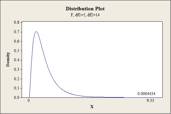
Software procedure:
- Click on Graph, select View Probability and click OK.
- Select F, enter 5 in numerator df and 14 in denominator df.
- Under Shaded Area Tab select X value under Define Shaded Area By and select Right tail.
- Choose X value as 9.33.
- Click OK.
Output obtained from MINITAB is given below:
Conclusion:
The P-value is 0.000 and the level of significance is 0.01.
The P-value is lesser than the level of significance.
That is
Thus, the null hypothesis is rejected.
Hence, there is sufficient evidence to conclude that there is ause of linear relationship between specific gravity and at least one of the five predictors at 1% level of significance.
b.
Calculate the adjusted
b.
Answer to Problem 56E
The adjusted
The adjusted
Explanation of Solution
Given info:
The
Calculation:
Adjusted
Adjusted
Substitute n as 20,k as 5,
Thus, the adjusted
Adjusted
Substitute n as 20, k as 4,
Thus, the adjusted
c.
Identify whether the data suggests that variables
Test the hypothesis to see whether the variables
c.
Answer to Problem 56E
Yes, the data suggests that variables
There issufficient evidence to conclude the variables
Explanation of Solution
Given info:
The
Calculation:
After dropping the three variables
The test hypotheses are given below:
Null hypothesis:
That is, there is no use of linear relationship betweenspecific gravity and at least one of the predictors, percentage of springwood and light absorption in summerwood.
Alternative hypothesis:
That is, there is use of linear relationship between specific gravity and at least one of the predictors, percentage of springwood and light absorption in summerwood.
From the
Similarly, the sum of squares due to error for the reduced model
Test statistic:
Where,
n represents the total number of observations.
k represents the number of predictors on the full model.
l represents the number of predictors on the reduced model.
Substitute 0.004542for
Critical value:
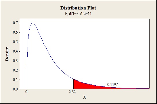
Software procedure:
- Click on Graph, select View Probability and click OK.
- Select F, enter 3 in numerator df and 14 in denominator df.
- Under Shaded Area Tab select Probability under Define Shaded Area By and select Right tail.
- Choose X Value as 2.32.
- Click OK.
Output obtained from MINITAB is given below:
Conclusion:
The P-value is 0.1197 and the level of significance is 0.05.
The P-value is lesser than the level of significance.
That is,
Thus, the null hypothesis is not rejected.
Hence, there is no sufficient evidence to conclude that there is a use of linear relationship betweenspecific gravity and at least one of the predictor percentage of springwood and light absorption in summerwood at 5% level of significance.
Thus, the variables
d.
Predict the value of specific gravity when the percentage of springwood is 50 and percentage of light absorption in summerwood is 90.
d.
Answer to Problem 56E
The estimated value for specific gravity when the percentage of springwood is 50 and percentage of light absorption in summerwood is 90 is 0.5386.
Explanation of Solution
Given info:
The mean and standard deviation for the variable
The estimated regression equation after standardization is
Calculation:
The standardized values
Where,
The standardized value when mean and standard deviation for the variable
Thus, the value of
The standardized value when the mean and standard deviation for the variable
Thus, the value of
The estimated value for specific gravity is,
Thus, the estimated value for specific gravity when the percentage of springwood is 50 and percentage of light absorption in summerwood is 90 is 0.5386.
e.
Find the 95% confidence interval for the estimated coefficient of
e.
Answer to Problem 56E
The 95% confidence interval for the estimated coefficient of
Explanation of Solution
Calculation:
95% confidence interval:
The confidence interval is calculated using the formula:
Where,
n is the total number of observations.
k is the total number of predictors in the model.
Critical value:
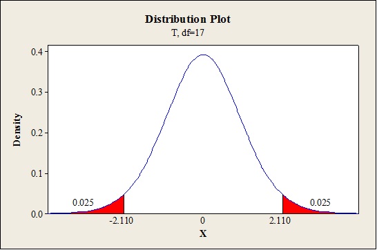
Software procedure:
Step-by-step procedure to find the critical value is given below:
- Click on Graph, select View Probability and click OK.
- Select t, enter 17 as Degrees of freedom, in Shaded Area Tab select Probability under Define Shaded Area By and choose Both tails.
- Enter Probability value as 0.05.
- Click OK.
Output obtained from MINITAB is given below:
The 95% confidence interval is given below:
Thus, the 95% confidence interval for the estimated coefficient of
f.
Find the estimated coefficient and estimated standard deviation of
f.
Answer to Problem 56E
The estimated coefficient of
The estimated standard deviation of
Explanation of Solution
Given info:
Use the information given in part (d) and (e).
Calculation:
The estimated regression equation for standardized model is,
The estimated coefficient of
Thus, the estimated coefficient of
The estimate for
The estimated standard deviation for
Thus, the estimated standard deviation of
g.
Find the 95% prediction interval for the specific gravity when the percentage of spring wood is 50.5 and percentage of light absorption in summerwood is 88.9.
g.
Answer to Problem 56E
The 95% prediction interval for the specific gravity when the percentage of spring wood is 50.5 and percentage of light absorption in summerwood is 88.9 is(0.489, 0.575).
Explanation of Solution
Given info:
The estimated standard deviation for the model with two predictors is 0.02001. The estimated standard deviation for the predicated value when the coefficients
Calculation:
The predicted value for the specific gravity when the percentage of spring wood is 50.5 and percentage of light absorption in summerwood is 88.9 is calculated as follows:
Thus, the predicted value for the specific gravity when the percentage of spring wood is 50.5 and percentage of light absorption in summerwood is 88.9 is 0.532.
95% prediction interval:
The confidence interval is calculated using the formula:
Where,
n is the total number of observations.
k is the total number of predictors in the model.
s is the overall standard deviation obtained after fitting the model.
Critical value:
Software procedure:
Step-by-step procedure to find the critical value is given below:
- Click on Graph, select View Probability and click OK.
- Select t, enter 17 as Degrees of freedom, in Shaded Area Tab select Probability under Define Shaded Area By and choose Both tails.
- Enter Probability value as 0.05.
- Click OK.
Output obtained from MINITAB is given below:
The 95% prediction interval is given below:
Thus, the 95% prediction interval for the specific gravity when the percentage of spring wood is 50.5 and percentage of light absorption in summerwood is 88.9 is (0.489,0.575).
Want to see more full solutions like this?
Chapter 13 Solutions
Probability and Statistics for Engineering and the Sciences


- An article in the Journal of Quality Technology (Vol. 13, No. 2, 1981, pp. 111–114) describes an experimentthat investigates the effects of four bleaching chemicals on pulp brightness. These four chemicals wereselected at random from a large population of potential bleaching agents. The data are as follows:a. Test the significance of these chemical types with α=0.05.b. If proven significant, perform a multiple comparison method using Fisher’s LSDarrow_forwardA study on the oxygen consumption rate (OCR) of sea cucumbers involved a random sample of size 12 at 15oC and a second random sample of size 5 kept at 18oC. To test the hypothesis that this range of temperature had no effect on the OCR, what is the degrees of freedom for a two-sample t-test?arrow_forwardBased on a survey of a random sample of 900 adults in the United States, a journalist reports that A random sample of 100 movie goers was asked to state his or her gender and favorite soft drink available at the local movie theater. The results appear in the table below. Is there a relationship between gender and soft drink preference? Coke Diet Coke Sprite Male 23 11 12 Female 16 28 10 To analyze the results, which of the following tests is most appropriate? A)Chi-square test of independence B)Chi-square test of homogeneity C)Two sample t-test D)Matched pair t-test E)Chi-square goodness of fitarrow_forward
- The dry shear strength of birch plywood bonded with different resin glues was studied with a completely randomized designed experiment. Here are the data: Glue A (102; 58; 45; 79; 68; 63; 117) Glue C (100; 102; 80; 119) Glue F (220; 243; 189; 176; 176). What is the F critical value at the 2.5% significance levelarrow_forwardThe article “Hydrogeochemical Characteristics of Groundwater in a Mid-Western CoastalAquifer System” (S. Jeen, J. Kim, et al., Geosciences Journal, 2001:339–348) presentsmeasurements of various properties of shallow groundwater in a certain aquifer system inKorea. Following are measurements of electrical conductivity (in microsiemens percentimeter) for 23 water samples.2099 528 2030 1350 1018 384 14991265 375 424 789 810 522 513488 200 215 486 257 557 260461 500Find the mean.Find the standard deviation.Find the median.Construct a dotplot.Find the 10% trimmed mean.Find the first quartile.Find the third quartile.Find the interquartile range.Construct a boxplot.Which of the points, if any, are outliers?If a histogram were constructed, would it be skewed to the left, skewed to the right, orapproximately symmetric?arrow_forwardLactation promotes a temporary loss of bone mass to provide adequate amounts of calcium for milk production. The paper “Bone Mass Is Recovered from Lactation to Postweaning in Adolescent Mothers with Low Calcium Intakes” (Amer. J. of Clinical Nutr., 2004: 1322–1326) gave the following data on total body bone mineral content (TBBMC) (g) for a sample both during lactation (L) and in the postweaning period (P). SubjectL 1928 2549 2825 1924 1628 2175 2114 2621 1843 2541P 2126 2885 2895 1942 1750 2184 2164 2626 2006 2627 Does the data suggest that true average total body bone mineral content during postweaning exceeds that during lactation by more than 25 g? State and test the appropriate hypotheses using a significance level of .05.arrow_forward
- The article “Structural Performance of Rounded Dovetail Connections Under Different Loading Conditions” (T. Tannert, H. Prion, and F. Lam, Can J Civ Eng, 2007:1600–1605) describes a study of the deformation properties of dovetail joints. In one experiment, 10 rounded dovetail connections and 10 double rounded dovetail connections were loaded until failure. The rounded connections had an average load at failure of 8.27 kN with a standard deviation of 0.62 kN. The double-rounded connections had an average load at failure of 6.11 kN with a standard deviation of 1.31 kN. Can you conclude that the mean load at failure is greater for rounded connections than for double-rounded connections?arrow_forwardA group of high-risk automobile drivers (with three moving violations in one year) are required, according to random assignment, either to attend a traffic school or to perform supervised volunteer work. During the subsequent five-year period, these same drivers were cited for the following number of moving violations: NUMBER OF MOVING VIOLATIONS TRAFFIC SCHOOL VOLUNTEER WORK 0 26 0 7 15 4 9 1 7 1 0 14 2 6 23 10 7 8 Why might the Mann–Whitney U test be preferred to the t test for these data? Use U to test the null hypothesis at the .05 level of significance. Specify the approximate p-value for this test result.arrow_forwardIn a breeding experiment, chicken with white feathers, small comb were mated and the offspring categories white feathers, small comb (WS), white feathers. large comb (WL), dark feathers, small comb (DS) and dark feathers, large comb (DL) were expected to follow the ratio 9:3:3:1 the researcher observed that there were 100 WS, 32 WL, 40 DS and 20 DL offspring. In order to test if the observed frequencies follow the expected ratio, what should be the hull hypothesis?A. P(WS) = 100/192, P(WL) = 32/192, P(DS) = 40/192 , P(DL) = 20/192 B. P(WS) = 100 , P(WL) = 32, P(DS) = 40, P(DL) = 20 C. P(WS) = 9/16 , P(WL) = 3/16, P(DS) = 3/16, P(DL) = 1/16 D. P(WS) = 9, P(WL) = 3, P(DS) = 3 , P(DL) = 1 2. In Problem 1, what would be the degree of freedom for an appropriate test?A.2 B.3 C.4 D.1 3. What is the value of the computed test statistic in problem 1? A.7.81 B.3.84 C.6.81 D.5.99 5.What would be the p-value for this test in problem 1? A.0.28 B.0.05 C.0.08 D. 0.11 6. At 5-% level of significance,…arrow_forward
- A random sample of 50 suspension helmets used by motorcycle riders and automobile race-car drivers was subjected to an impact test, and on 18 of these helmets some damage was observed.arrow_forwardA sample of men and women who had passed their driver's test either the first time or the second time were surveyed, with the following results: Results of the driving testGender First time Second timeMen 126 211Women 135 178a) Do these data suggest that there is a relationship between gender and the passing of their driver’s test from which the present sample was drawn? Let alpha=.05arrow_forwardSpecimens of three different types of rope wire wereselected, and the fatigue limit (MPa) was determined foreach specimen, resulting in the accompanying data.Type 1 350 350 350 358 370 370 370 371371 372 372 384 391 391 392Type 2 350 354 359 363 365 368 369 371373 374 376 380 383 388 392Type 3 350 361 362 364 364 365 366 371377 377 377 379 380 380 392a. Construct a comparative boxplot, and comment onsimilarities and differences.b. Construct a comparative dotplot (a dotplot for eachsample with a common scale). Comment on similaritiesand differences.c. Does the comparative boxplot of part (a) give aninformative assessment of similarities and differences?Explain your reasoning.arrow_forward
 MATLAB: An Introduction with ApplicationsStatisticsISBN:9781119256830Author:Amos GilatPublisher:John Wiley & Sons Inc
 Probability and Statistics for Engineering and th...StatisticsISBN:9781305251809Author:Jay L. DevorePublisher:Cengage Learning
 Statistics for The Behavioral Sciences (MindTap C...StatisticsISBN:9781305504912Author:Frederick J Gravetter, Larry B. WallnauPublisher:Cengage Learning
 Elementary Statistics: Picturing the World (7th E...StatisticsISBN:9780134683416Author:Ron Larson, Betsy FarberPublisher:PEARSON
 The Basic Practice of StatisticsStatisticsISBN:9781319042578Author:David S. Moore, William I. Notz, Michael A. FlignerPublisher:W. H. Freeman
 Introduction to the Practice of StatisticsStatisticsISBN:9781319013387Author:David S. Moore, George P. McCabe, Bruce A. CraigPublisher:W. H. Freeman