Concept explainers
Videos
a.
Make the
Find the independent variable that has the strongest correlation with the dependent variable.
Explain whether the strong correlation between some independent variables indicate any problem.
a.
Answer to Problem 20CE
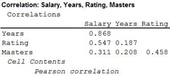
The correlation matrix is obtained as,
The independent variable that has the strongest correlation with the dependent variable is “Years of experience”.
Explanation of Solution
Multiple linear regression model:
A multiple linear regression model is given as
Here, a is the intercept term of the regression model, that is, the value of predicted value of y when X’s are 0 and
Dummy variable:
A dichotomous variable is defined as a dummy variable, where one outcome is defined as 1 another as 0.
In the given problem the predicted dependent variable y is the salary. The years of experience, the Principal’s rating, and the Master’s Degree, are defined as
The independent random variable
Hence,
Step by step procedure to obtain the correlation matrix using MINITAB software is given below:
- Choose Stat > Basic Statistics > Correlation.
- Select Years, Rating and Masters under Variables tab.
- Click OK.
The MINITAB output is obtained.
According to the obtained output there is a strongest correlation between the independent variable “Years” and the dependent variable “Salary”. The correlation coefficient between “Years” and “Salary” is 0.868.
Thus, it implies that as the years of experience increases the salary also increases.
Multicollinearity:
In a multiple regression model, when there is high correlation between two or more independent variables, then multicollinearity occurs.
The correlation between the independent variables “Rating” and “Masters” is 0.458, which is maximum among the correlation between the independent variables.
Thus, there is no chance of occurrence of multicollinearity in the regression model.
b.
Find the regression equation.
Find the estimated salary for a teacher with 5 years’ experience, a rating by the principal of 60 and no master’s degree.
b.
Answer to Problem 20CE
The regression equation is
The estimated salary for a teacher with 5 years’ experience, a rating by the principal of 60 and no master’s degree is $33,651.
Explanation of Solution
Calculation:
Step by step procedure to obtain the regression equation using MINITAB software:
- Choose Stat > Regression > Regression > Fit Regression Model.
- Under Responses, enter the column of Salary.
- Under Continuous predictors, enter the columns of Years, Rating and Masters.
- Click OK.
Output using MINITAB software is given below:
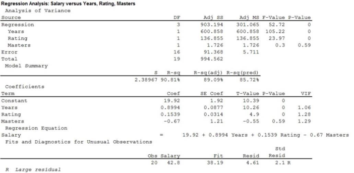
Thus, the regression equation is
Now, substitute
Hence,
Thus, the estimated salary for a teacher with 5 years’ experience, a rating by the principal of 60 and no master’s degree is $33,651.
c.
Perform a global hypothesis test to check whether any of the regression coefficients differ from zero at 0.05 level of significance.
c.
Answer to Problem 20CE
There is strong evidence that any of the regression coefficient differ from 0 at 0.05 significance level.
Explanation of Solution
Calculation:
Consider that y is dependent variable and
State the hypotheses:
Null hypothesis:
That is, the model is not significant.
Alternative hypothesis:
That is, the model is significant.
In case of global test the F test statistic is defined as,
According to the output in Part (b) the value of F statistic is 52.72 with numerator degrees of freedom 3 and denominator degrees of freedom 16.
The level of significance is
Decision rule:
- If
- Otherwise failed to reject the null hypothesis.
Conclusion:
Here, p-value corresponding to the global test is 0.
Hence,
That is, the p-value is less than the level of significance.
Therefore, reject the null hypothesis.
Hence, it can be concluded that any of the regression coefficient differ from 0 at 0.05 significance level.
d.
Perform individual tests of each independent variable at 0.05 significance level.
Explain whether any of the independent variable will be eliminated.
d.
Answer to Problem 20CE
There is no significant relation between y and
The independent random variable “Master’s degree” can be eliminated.
Explanation of Solution
Calculation:
For independent variable
Consider that
State the hypotheses:
Null hypothesis:
That is, there is no significant relationship between y and
Alternative hypothesis:
That is, there is significant relationship between y and
In case of individual regression coefficient test the t test statistic is defined as,
According to the output in Part (a) the t statistic value corresponding to
Conclusion:
Here, p-value corresponding to the “Years of experience”
Hence,
That is, the p-value is less than the level of significance.
Therefore, reject the null hypothesis.
Hence, it can be concluded that there is significant relationship between y and
For independent variable
Consider that
State the hypotheses:
Null hypothesis:
That is, there is no significant relationship between y and
Alternative hypothesis:
That is, there is significant relationship between y and
According to the output in Part (a) the value of t test statistic corresponding to
Conclusion:
Here, p-value corresponding to the “Principal’s rating”
Hence,
That is, the p-value is less than the level of significance.
Therefore, reject the null hypothesis.
Hence, it can be concluded that there is significant relationship between y and
For independent variable
Consider that
State the hypotheses:
Null hypothesis:
That is, there is no significant relationship between y and
Alternative hypothesis:
That is, there is significant relationship between y and
According to the output in Part (a) the value of t test statistic corresponding to
Conclusion:
Here, p-value corresponding to the income
Hence,
That is, the p-value is greater than the level of significance.
Therefore, fail to reject the null hypothesis.
Hence, it can be concluded that there is no significant relationship between y and
As there are no significant relationship between the dependent variable and the independent variable
Hence, it can be said that there is no significant relationship between the salary and the Master’s degree. Thus, it is better to omit the independent random variable “Master’s degree”.
e.
Perform the
e.
Explanation of Solution
Calculation:
The regression analysis is performed after omitting the independent variable Master’s degree.
Step by step procedure to obtain the regression equation using MINITAB software:
- Choose Stat > Regression > Regression > Fit Regression Model.
- Under Responses, enter the column of Salary.
- Under Continuous predictors, enter the columns of Years, and Rating
- Choose Graphs.
- Under Residual plot select Histogram of residuals and Residual Versus fit.
- Click OK.
- Choose Storage.
- Under Regression storage select Residuals.
- Click OK
- Click OK.
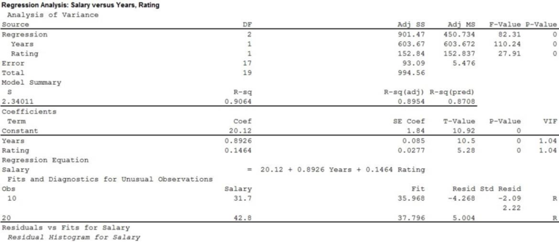
Output using MINITAB software is given below:
| Residuals |
| –1.2802 |
| 2.726697 |
| –0.0664 |
| 0.711748 |
| –2.0206 |
| 0.676788 |
| 2.725551 |
| 2.531216 |
| 0.795113 |
| –4.26789 |
| 0.300234 |
| –0.41968 |
| –1.14257 |
| 0.284365 |
| –2.38135 |
| –2.67229 |
| 1.368873 |
| –2.06188 |
| –0.81143 |
| 5.00372 |

Thus, the regression equation is
Global test:
State the hypotheses:
Null hypothesis:
That is, the model is not significant.
Alternative hypothesis:
That is, the model is significant.
In case of global test the F test statistic is defined as,
According to the output in the value of F statistic is 82.31 with numerator degrees of freedom 2 and denominator degrees of freedom 17.
Conclusion:
Here, p-value corresponding to the global test is 0.
Hence,
That is, the p-value is less than the level of significance.
Therefore, reject the null hypothesis.
Hence, it can be concluded that any of the regression coefficient differ from 0 at 0.05 significance level.
Individual test:
For independent variable
Null hypothesis:
That is, there is no significant relationship between y and
Alternative hypothesis:
That is, there is significant relationship between y and
According to the output the t statistic value corresponding to
Conclusion:
Here, p-value corresponding to the “Years of experience”
Hence,
That is, the p-value is less than the level of significance.
Therefore, reject the null hypothesis.
Hence, it can be concluded that there is significant relationship between y and
For independent variable
Null hypothesis:
That is, there is no significant relationship between y and
Alternative hypothesis:
That is, there is significant relationship between y and
According to the output the value of t test statistic corresponding to
Conclusion:
Here, p-value corresponding to the “Principal’s rating”
Hence,
That is, the p-value is less than the level of significance.
Therefore, reject the null hypothesis.
Hence, it can be concluded that there is significant relationship between y and
f.
Find the residuals for the equation of Part (e).
Find a stem-and-leaf plot or a histogram to verify whether the distribution of the residuals is approximately normal.
f.
Explanation of Solution
Calculation:
From Part (e), the residuals are obtained as,
| Residuals |
| –1.2802 |
| 2.726697 |
| –0.0664 |
| 0.711748 |
| –2.0206 |
| 0.676788 |
| 2.725551 |
| 2.531216 |
| 0.795113 |
| –4.26789 |
| 0.300234 |
| –0.41968 |
| –1.14257 |
| 0.284365 |
| –2.38135 |
| –2.67229 |
| 1.368873 |
| –2.06188 |
| –0.81143 |
| 5.00372 |
Histogram:
From Part (e), the histogram is obtained as,
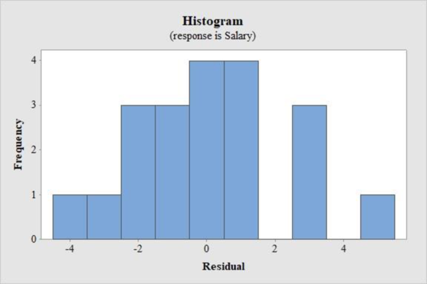
Assumption of normality from histogram:
- The majority of the observation in the middle and centered on the mean of 0.
- There are lower frequencies on the tails of the distributions.
According to the given histogram, the most of the observations are centered on the mean of 0 and there are less frequencies on the tails of the distributions. However, it is roughly symmetric.
Hence, the normality assumptions appear somehow.
g.
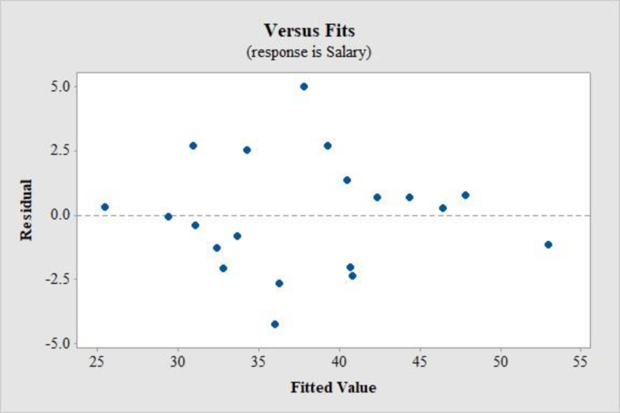
Plot the residual plot.
Explain whether the plot reveals any violations of assumptions of regression.
g.
Explanation of Solution
From Part (e), the residual plot is obtained as,

Assumption for residual analysis for the regression model:
- The plot of the residuals vs. the observed values of the predictor variable should fall roughly in a horizontal band and symmetric about x-axis.
- For a normal probability plot, residuals should be roughly linear.
- There should not be any observable pattern.
According to the given residual plot, the points are roughly in a horizontal band and more or less symmetric about x-axis. Moreover, there is no particular pattern in the residual plot. A complete haphazard and random nature has observed.
Hence, the assumptions of the residual plot are not violated.
Want to see more full solutions like this?
Chapter 14 Solutions
EBK STATISTICAL TECHNIQUES IN BUSINESS


 College Algebra (MindTap Course List)AlgebraISBN:9781305652231Author:R. David Gustafson, Jeff HughesPublisher:Cengage Learning
 Glencoe Algebra 1, Student Edition, 9780079039897...AlgebraISBN:9780079039897Author:CarterPublisher:McGraw Hill