Videos
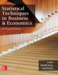
Great Plains Distributors, Inc. sells roofing and siding products to home improvement retailers, such as Lowe’s and Home Depot, and commercial contractors. The owner is interested in studying the effects of several variables on the sales volume of fiber-cement siding products.
The company has 26 marketing districts across the United States. In each district, it collected information on the following variables: sales volume (in thousands of dollars), advertising dollars (in thousands), number of active accounts, number of competing brands, and a rating of market potential.
Conduct a multiple
- a. Draw a
scatter diagram comparing sales volume with each of the independent variables. Comment on the results. - b. Develop a
correlation matrix. Do you see any problems? Does it appear there are any redundant independent variables? - c. Develop a regression equation. Conduct the global test. Can we conclude that some of the independent variables are useful in explaining the variation in the dependent variable?
- d. Conduct a test of each of the independent variables. Are there any that should be dropped?
- e. Refine the regression equation so the remaining variables are all significant.
- f. Develop a histogram of the residuals and a normal probability plot. Are there any problems?
- g. Determine the variance inflation factor for each of the independent variables. Are there any problems?
a.
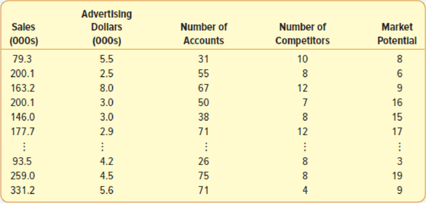
Make a scatter diagram that compares sales with each of the independent variables.
Explain the results.
Answer to Problem 23CE
The scatter diagram is obtained below,
Explanation of Solution
Step by step procedure to obtain the correlation matrix using MINITAB software is given below:
- Choose Graph > Matrix plot.
- Under Each Y versus each X, select Simple.
- Under Y variable select the column of Sales.
- Under X variables select the columns of Ad Dollars, Number of accounts, Number of Competitors, and Potential.
- Click OK.
The MINITAB output is obtained.
According to the output, as the number of competitors increases the sales decreases. In other hand, as the number of accounts and the rating of market potential increases, the sales also increase. However, there is no linear relationship between the Ad Dollars with the sales.
b.
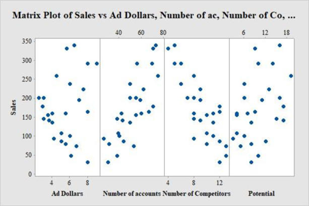
Make the correlation matrix.
Explain whether there is any problem due to redundant independent variables.
Answer to Problem 23CE
The correlation matrix is obtained as,
Explanation of Solution
Multiple linear regression model:
A multiple linear regression model is given as
Here, a is the intercept term of the regression model, that is, the value of predicted value of y when X’s are 0 and
In the given problem the predicted dependent variable y is the sales. The years of advertising dollars, the number of accounts, the number of competitors and the rating of market potential, are defined as
Step by step procedure to obtain the correlation matrix using MINITAB software is given below:
- Choose Stat > Basic Statistics > Correlation.
- Select the columns of Sales, Ad Dollars, Number of accounts, Number of Competitors, and Potential under Variables tab.
- Click OK.
The MINITAB output is obtained.
Multicollinearity:
In a multiple regression model, when there is high correlation between two or more independent variables, then multicollinearity occurs.
There is moderate correlation between the independent variables “Potential” and “Number of Accounts”.
Thus, there is no chance of occurrence of multicollinearity in the regression model.
c.
Find the regression equation and perform a global test.
Answer to Problem 23CE
The regression equation is
Some of the independent variables are useful in explaining the variation in the dependent variable at 0.05 significance level.
Explanation of Solution
Calculation:
Step by step procedure to obtain the regression equation using MINITAB software:
- Choose Stat > Regression > Regression > Fit Regression Model.
- Under Responses, enter the column of Sales.
- Under Continuous predictors, enter the columns of Ad Dollars, Number of accounts, Number of Competitors, and Potential.
- Click OK.
Output using MINITAB software is given below:
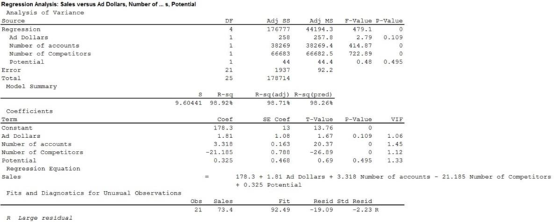
Thus, the regression equation is
Consider that y is dependent variable and
State the hypotheses:
Null hypothesis:
That is, the model is not significant.
Alternative hypothesis:
That is, the model is significant.
In case of global test the F test statistic is defined as,
According to the output the value of F statistic is 479.1 with numerator degrees of freedom 4 and denominator degrees of freedom 21.
Consider that, the level of significance is
Decision rule:
- If
- Otherwise failed to reject the null hypothesis.
Conclusion:
Here, p-value corresponding to the global test is 0.
Hence,
That is, the p-value is less than the level of significance.
Therefore, reject the null hypothesis.
Hence, it can be concluded that some of the independent variables are useful in explaining the variation in the dependent variable at 0.05 significance level.
d.
Perform individual tests of each independent variables.
Explain whether any variable should be dropped.
Answer to Problem 23CE
There is significant relationship between y and
It is better to drop these two variables
Explanation of Solution
Calculation:
For independent variable
Consider that
State the hypotheses:
Null hypothesis:
That is, there is no significant relationship between y and
Alternative hypothesis:
That is, there is significant relationship between y and
In case of individual regression coefficient test the t test statistic is defined as,
According to the output in Part (c) the t statistic value corresponding to
Conclusion:
Here, p-value corresponding to the “Ad Dollars”
Hence,
That is, the p-value is greater than the level of significance.
Therefore, fail to reject the null hypothesis.
Hence, it can be concluded that there is no significant relationship between y and
For independent variable
Consider that
State the hypotheses:
Null hypothesis:
That is, there is no significant relationship between y and
Alternative hypothesis:
That is, there is significant relationship between y and
According to the output in Part (c) the value of t test statistic corresponding to
Conclusion:
Here, p-value corresponding to the “Number of accounts”
Hence,
That is, the p-value is less than the level of significance.
Therefore, reject the null hypothesis.
Hence, it can be concluded that there is significant relationship between y and
For independent variable
Consider that
State the hypotheses:
Null hypothesis:
That is, there is no significant relationship between y and
Alternative hypothesis:
That is, there is significant relationship between y and
According to the output in Part (c) the value of t test statistic corresponding to
Conclusion:
Here, p-value corresponding to the “Number of competitors”
Hence,
That is, the p-value is less than the level of significance.
Therefore, reject the null hypothesis.
Hence, it can be concluded that there is significant relationship between y and
For independent variable
Consider that
State the hypotheses:
Null hypothesis:
That is, there is no significant relationship between y and
Alternative hypothesis:
That is, there is significant relationship between y and
According to the output in Part (c) the value of t test statistic corresponding to
Conclusion:
Here, p-value corresponding to the “Potential”
Hence,
That is, the p-value is greater than the level of significance.
Therefore, fail to reject the null hypothesis.
Hence, it can be concluded that there is no significant relationship between y and
Hence, it can be said that as there is no significant relationship between “Sales” and “Ad Dollars” and between “Sales” and “Potential”, thus it is better to omit these two variables and perform the regression analysis using “Number of accounts” and “Number of competitors” as independent variables.
e.
Refine the regression equation so the remaining variables are all significant.
Answer to Problem 23CE
The refined regression equation is
Explanation of Solution
Calculation:
In this part the dependent variable is sales (y) and the independent variables are the number of accounts
Step by step procedure to obtain the regression equation using MINITAB software:
- Choose Stat > Regression > Regression > Fit Regression Model.
- Under Responses, enter the column of Sales.
- Under Continuous predictors, enter the columns of Number of accounts, and Number of Competitors.
- Choose Graphs.
- Under Residual plot select Histogram of residuals, Normal probability plot of residuals.
- Click OK.
- Click OK.
Output using MINITAB software is given below:
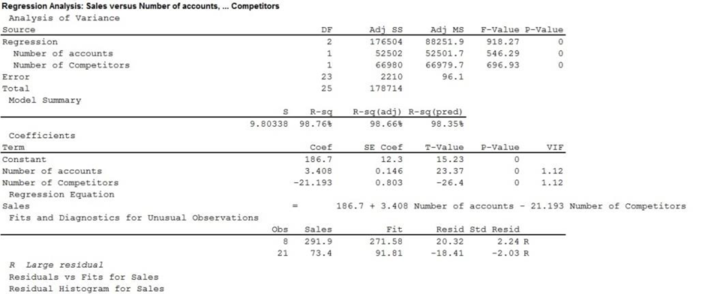

Hence, the regression equation is
For independent variable
Consider that
State the hypotheses:
Null hypothesis:
That is, there is no significant relationship between y and
Alternative hypothesis:
That is, there is significant relationship between y and
According to the output the t statistic value corresponding to
Conclusion:
Here, p-value corresponding to the “Number of Accounts”
Hence,
That is, the p-value is less than the level of significance.
Therefore, reject the null hypothesis.
Hence, it can be concluded that there is significant relationship between y and
For independent variable
Consider that
State the hypotheses:
Null hypothesis:
That is, there is no significant relationship between y and
Alternative hypothesis:
That is, there is significant relationship between y and
According to the output in the value of t test statistic corresponding to
Conclusion:
Here, p-value corresponding to the “Number of competitors”
Hence,
That is, the p-value is less than the level of significance.
Therefore, reject the null hypothesis.
Hence, it can be concluded that there is significant relationship between y and
Hence, it can be said that as there is significant relationship between “Sales” and “Number of accounts” and “Number of competitors”.
f.
Provide a histogram and normal probability plot for residuals.
Also explain whether there are any problems.
Explanation of Solution
Calculation:
Histogram:
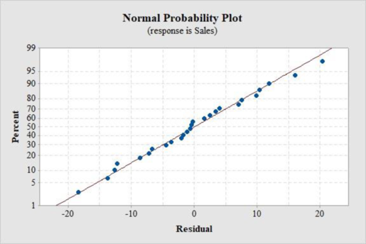
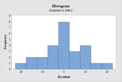
From Part (e), the histogram and normal probability plot is obtained as,

Assumption of normality from histogram:
- The majority of the observation in the middle and centered on the mean of 0.
- There are lower frequencies on the tails of the distributions.
According to the given histogram, the most of the observations are centered on the mean of 0 and there are less frequencies on the tails of the distributions. In addition, it can be considered as perfect symmetric.
According to the normal probability plot, all of the residuals are linear.
Hence, there are no problems in normality assumptions.
g.
Find the variation inflection factor for each of the independent variables.
Explain whether there is any problem.
Explanation of Solution
Variation inflation factor(VIF):
The variation inflation factor is defined as,
It is used to detect multicollinearity in the regression. If
From Part (e), the variation inflection factor corresponding to both variables are 1.12, which is less than 10.
Hence, there is no presence of multicollinearity.
Want to see more full solutions like this?
Chapter 14 Solutions
EBK STATISTICAL TECHNIQUES IN BUSINESS


- Rebecca Chory, Ph.D., now an associate professor of communication at West Virginia University, began studying the effect of such portrayals on patients' attitudes toward physicians. Using a survey of 300 undergraduate students, she compared perceptions of physicians in 1992—the end of the era when physicians were shown as all-knowing, wise father figures—with those in 1999, when shows such as ER and Chicago Hope (1994–2000) were continuing the transformation to showing the private side and lives of physicians, including vivid demonstrations of their weaknesses and insecurities. Dr. Chory found that, regardless of the respondents' personal experience with physicians, those who watched certain kinds of television had declining perceptions of physicians' composure and regard for others. Her results indicated that the more prime time physician shows that people watched in which physicians were the main characters, the more uncaring, cold, and unfriendly the respondents thought physicians…arrow_forwardRebecca Chory, Ph.D., now an associate professor of communication at West Virginia University, began studying the effect of such portrayals on patients' attitudes toward physicians. Using a survey of 300 undergraduate students, she compared perceptions of physicians in 1992—the end of the era when physicians were shown as all-knowing, wise father figures—with those in 1999, when shows such as ER and Chicago Hope (1994–2000) were continuing the transformation to showing the private side and lives of physicians, including vivid demonstrations of their weaknesses and insecurities. Dr. Chory found that, regardless of the respondents' personal experience with physicians, those who watched certain kinds of television had declining perceptions of physicians' composure and regard for others. Her results indicated that the more prime time physician shows that people watched in which physicians were the main characters, the more uncaring, cold, and unfriendly the respondents thought physicians…arrow_forwardThe St. Lucian Government is interested in predicting the number of weekly riders on the public buses using the following variables: Price of bus trips per week The population in the city The monthly income of riders Average rate to park your personal vehicle City Number of weekly riders Price per week Population of city Monthly income of riders Average parking rates per month 1 192,000 $15 1,800,000 $5,800 $50 2 190,400 $15 1,790,000 $6,200 $50 3 191,200 $15 1,780,000 $6,400 $60 4 177,600 $25 1,778,000 $6,500 $60 5 176,800 $25 1,750,000 $6,550 $60 6 178,400 $25 1,740,000 $6,580 $70 7 180,800 $25 1,725,000 $8,200 $75 8 175,200 $30 1,725,000 $8,600 $75 9 174,400 $30 1,720,000 $8,800 $75 10 173,920 $30 1,705,000 $9,200 $80 11 172,800 $30 1,710,000 $9,630 $80 12 163,200 $40 1,700,000 $10,570…arrow_forward
- The St. Lucian Government is interested in predicting the number of weekly riders on the public buses using the following variables: Price of bus trips per week The population in the city The monthly income of riders Average rate to park your personal vehicle City Number of weekly riders Price per week Population of city Monthly income of riders Average parking rates per month 1 192,000 $15 1,800,000 $5,800 $50 2 190,400 $15 1,790,000 $6,200 $50 3 191,200 $15 1,780,000 $6,400 $60 4 177,600 $25 1,778,000 $6,500 $60 5 176,800 $25 1,750,000 $6,550 $60 6 178,400 $25 1,740,000 $6,580 $70 7 180,800 $25 1,725,000 $8,200 $75 8 175,200 $30 1,725,000 $8,600 $75 9 174,400 $30 1,720,000 $8,800 $75 10 173,920 $30 1,705,000 $9,200 $80 11 172,800 $30 1,710,000 $9,630 $80 12 163,200 $40 1,700,000 $10,570…arrow_forwardThe St. Lucian Government is interested in predicting the number of weekly riders on the public buses using the following variables: Price of bus trips per week The population in the city The monthly income of riders Average rate to park your personal vehicle City Number of weekly riders Price per week Population of city Monthly income of riders Average parking rates per month 1 192,000 $15 1,800,000 $5,800 $50 2 190,400 $15 1,790,000 $6,200 $50 3 191,200 $15 1,780,000 $6,400 $60 4 177,600 $25 1,778,000 $6,500 $60 5 176,800 $25 1,750,000 $6,550 $60 6 178,400 $25 1,740,000 $6,580 $70 7 180,800 $25 1,725,000 $8,200 $75 8 175,200 $30 1,725,000 $8,600 $75 9 174,400 $30 1,720,000 $8,800 $75 10 173,920 $30 1,705,000 $9,200 $80 11 172,800 $30 1,710,000 $9,630 $80 12 163,200 $40 1,700,000 $10,570…arrow_forwardShould large retailers offer banking services? Small community banks may be concerned about their future if more retailers enter the world of banking. Suppose that a market research company conducted a national survey for one retailer that is considering offering banking services to its customers. The respondents were asked to indicate the provider (bank, retail store, other) that they most likely would use for certain banking services (assuming that rate is not a factor). Is there a relationship between these two variables? Provider Service Bank Retail Store Other Checking account Savings account Home mortgage 100 85 30 45 25 10 10 45 80arrow_forward
- A study is conducted to determine the relationship between study hours and exam scores, what is the dependent variable in this scenario?arrow_forwardIn a study to see if there is a relationship between students’ consumption of alcoholic beverages and their grade point averages, the drinking behavior would be the presumed cause or ____________________________ variable and the grade point average would be the effect or ________________________________________ variable.arrow_forwardCity Hotel Room Rate ($) Entertainment ($) Boston 144 161 Denver 96 103 Nashville 88 103 New Orleans 112 143 Phoenix 89 100 San Diego 100 119 San Francisco 137 166 San Jose 93 138 Tampa 86 99 Concur Technologies, Inc., is a large expense-management company located in Redmond, Washington. The Wall Street Journal asked Concur to examine the data from 8.3 million expense reports to provide insights regarding business travel expenses. Their analysis of the data showed that New York was the most expensive city, with an average daily hotel room rate of $198 and an average amount spent on entertainment, including group meals and tickets for shows, sports, and other events, of $172. In comparison, the U.S. averages for these two categories were $89 for the room rate and $99 for entertainment. The table in the Excel Online file below shows the average daily hotel room rate and the amount spent on entertainment for a random sample of 9 of the 25 most visited U.S. cities (The…arrow_forward
- Under what circumstances could an independent variable in one study be a dependent variable in another study?arrow_forwardA researcher is interested in comparing the effectiveness of three popular diets for weightloss: The Paleo diet, Keto, and the Atkins diet. She randomly assigns participants to follow one of the three diet trends for 6 months, and then compares the amount of weight lost in each group. What is the Independent Variable and the Dependent Variable?arrow_forwardSuppose researchers at an abdominal transplant clinic are concerned about the rate of graft loss due to diabetes status prior to receiving a donor kidney. Research has shown that gender discordance, or receiving a gender from a donor of an opposite gender may increase the risk of both exposure and outcome after transplant. Assume the following tables represent the stratified analysis of the potential confounding variable. (9 points) Gender Discordance Graft Failure No Graft Failure Total Diabetes II 23 10 33 No Diabetes II 4 44 48 Total 27 54 81 Gender Concordance Graft Failure No Graft Failure Total Diabetes II 9 34 43 No Diabetes II 12 87 99 Total 21 121 142 A) Calculate the stratum specific estimates for the odds ratios in each strata. B) Observe the difference in the odds ratios. Based on observation alone, what are we likely to conclude regarding the relationship between outcome and exposure…arrow_forward
 Glencoe Algebra 1, Student Edition, 9780079039897...AlgebraISBN:9780079039897Author:CarterPublisher:McGraw Hill
 Big Ideas Math A Bridge To Success Algebra 1: Stu...AlgebraISBN:9781680331141Author:HOUGHTON MIFFLIN HARCOURTPublisher:Houghton Mifflin Harcourt