Introduction To Statistics And Data Analysis
6th Edition
ISBN: 9781337793612
Author: PECK, Roxy.
Publisher: Cengage Learning,
bartleby

Concept explainers

bartleby

Videos

Question
Book Icon
Chapter 14, Problem 63CR

a.

To determine

Test whether the linear relationship is useful or not at the 0.01 level of significance.

a.

Expert Solution
Check Mark

Answer to Problem 63CR

There is convincing evidence that the linear relationship is useful between y and at least one of the predictors at the 0.01 level of significance.

Explanation of Solution

Calculation:

It is given that variable y is the average language score, x1 is occupational index, x2 is median income, x3 is percentage of title I enrollment, x4 is Hispanic enrollment, x5 is logarithm of fourth-grade enrollment, x6 is prior test score, x7 is administrator teacher ratio, x8 is pupil teacher ratio, x9 is certified staff pupil ratio, and x10,x11 are the indicator variables for average teaching experience. The sample size is 88 and the number of variables (k) is 11.

1.

The model is y=α+β1x1+β2x2+...+β11x11+e.

2.

Null hypothesis:

H0:β1=β2=...=β11=0

That is, there is no useful linear relationship between y and any of the predictors.

3.

Alternative hypothesis:

Ha: At least one among βi's is not zero.

That is, there is a useful linear relationship between y and any of the predictors.

4.

Here, the significance level is α=0.01.

5.

Test statistic:

F=R2k(1R2)n(k+1)

Here, n is the sample size and k is the number of variables in the model.

6.

Assumptions:

Since there is no availability of original data to check the assumptions, there is a need to assume that the variables are related to the model, and the random deviation is distributed normally with mean 0 and the fixed standard deviation.

7.

Calculation:

The value of R2 is 0.64.

The value of F-test statistic is calculated as follows:

F=R2k(1R2)n(k+1)=0.6411(10.64)(88(11+1))=0.0580.3676=0.058×760.36=4.4080.36=12.24

8.

P-value:

Software procedure:

Step-by-step procedure to find the P-value using the MINITAB software:

  • Choose Graph > Probability Distribution Plot choose View Probability > OK.
  • From Distribution, choose ‘F’ distribution.
  • Enter the Numerator df as 11 and Denominator df as 76.
  • Click the Shaded Area tab.
  • Choose X Value and Right Tail for the region of the curve to shade.
  • Enter the X value as 12.24.
  • Click OK.

Output obtained using the MINITAB software is represented as follows:

Introduction To Statistics And Data Analysis, Chapter 14, Problem 63CR , additional homework tip  1

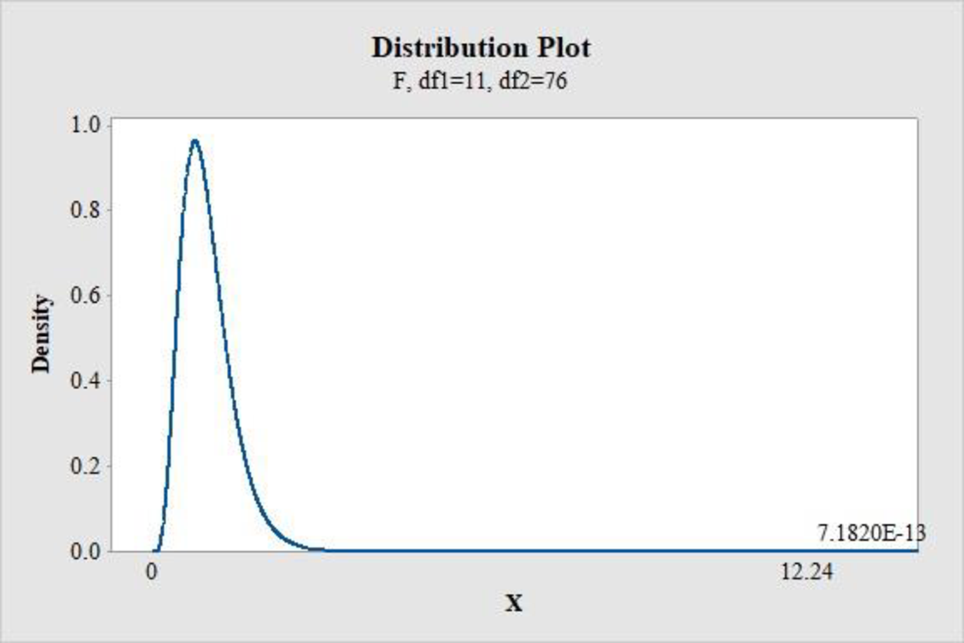
From MINITAB output, the P-value is 0.

9.

Conclusion:

If P-valueα, then reject the null hypothesis.

Therefore, the P-value of 0 is less than the 0.01 level of significance.

Hence, reject the null hypothesis.

Thus, there is convincing evidence that the linear relationship is useful between y and at least one of the predictors at the 0.01 level of significance.

b.

To determine

Calculate the value of adjusted R2.

b.

Expert Solution
Check Mark

Answer to Problem 63CR

The value of adjusted R2 is 0.5879.

Explanation of Solution

Calculation:

The formula for adjusted R2 is as follows:

Radj2=1(1R2)(n1n(k+1))

Substitute the value of R2 as 0.64, n as 88, and k as 11 in the adjusted R2 formula.

Radj2=1(1R2)(n1n(k+1))=1(10.64)(88188(11+1))=1(0.36)(8776)=10.4121=0.5879

Thus, the value of adjusted R2 is 0.5879.

c.

To determine

Calculate a 95% confidence interval for β1 and interpret it.

c.

Expert Solution
Check Mark

Answer to Problem 63CR

The 95% confidence interval for β1 is (0.1615,0.7545_).

Explanation of Solution

Calculation:

Here, β1 is the coefficient of variable x1.

Since there is no availability of original data to check the assumptions, there is a need to assume that the variables are related to the model, and the random deviation is distributed normally with mean 0 and the fixed standard deviation.

The formula for confidence interval for β1 is as follows:

b1±(t critical value)sb1.

Where, b1 is the estimated value of β1 and sb1 is the estimated standard deviation of b1.

Degrees of freedom:

df=n(k+1)=88(11+1)=8812=76

Software procedure:

Step-by-step procedure to find P-value using the MINITAB software:

  • Choose Graph > Probability Distribution Plot choose View Probability > OK.
  • From Distribution, choose ‘t’ distribution.
  • Enter the Degrees of freedom as 76.
  • Click the Shaded Area tab.
  • Choose Probability and Both Tails for the region of the curve to shade.
  • Enter the Probability value as 0.05.
  • Click OK.

Output obtained using the MINITAB software is represented as follows:

Introduction To Statistics And Data Analysis, Chapter 14, Problem 63CR , additional homework tip  2

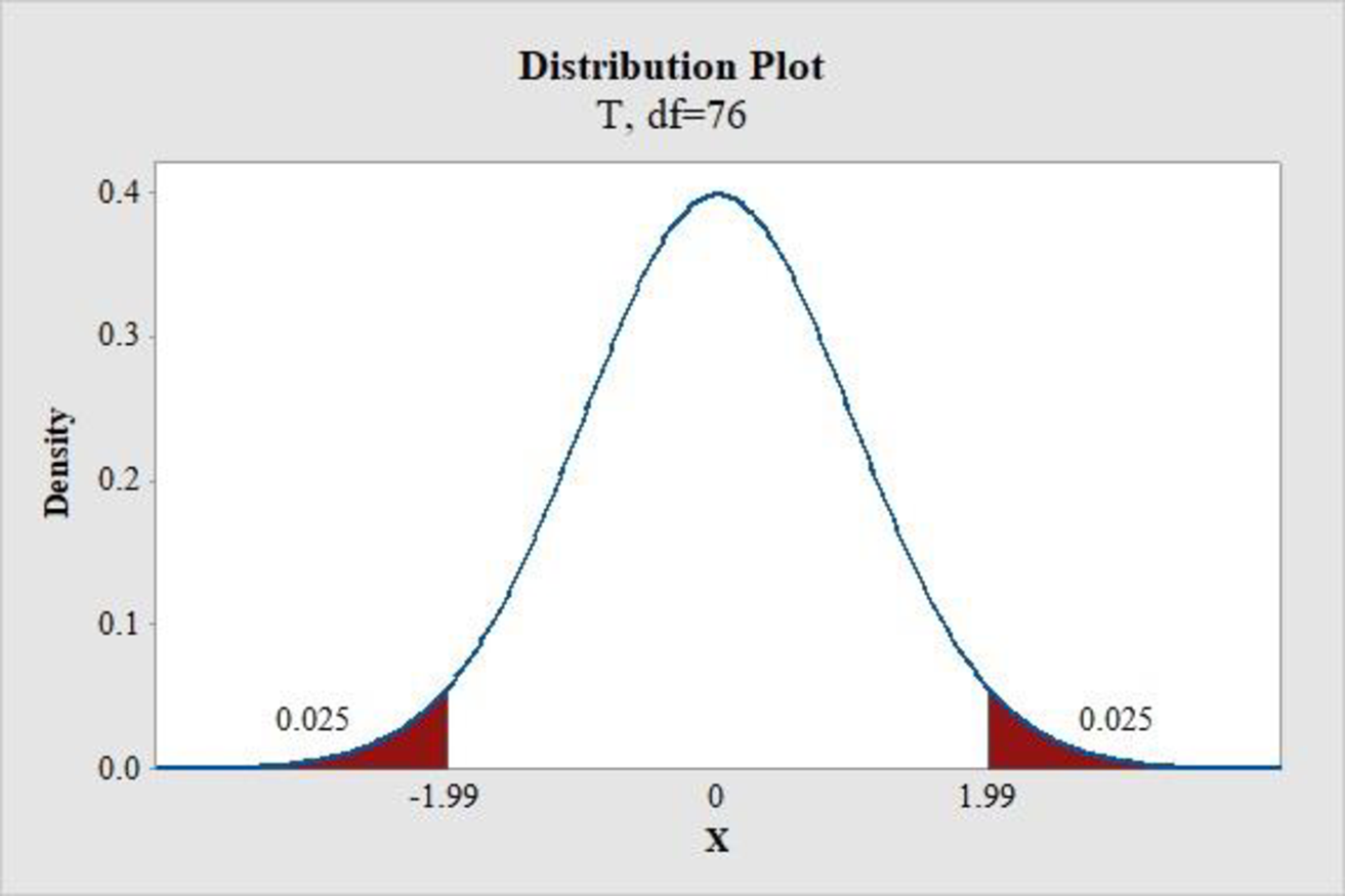
From the MINITAB output, the critical value is 1.99.

The value of sb1 is calculated as follows:

sb1=b1t1=0.4583.08=0.149

Here, the value of b1 is 0.458 and the value of sb1 is 0.149.

The 95% confidence interval for β1 is calculated as follows:

b1±(t critical value)sb1=0.458±(1.99)0.149=0.458±0.2965=(0.4580.2965,0.458+0.2965)=(0.1615,0.7545)

Thus, the 95% confidence interval for β1 is (0.1615,0.7545_).

Interpretation:

There is 95% confidence that the average increase in y associated with 1-unit increase in occupational index is between 0.1615 and 0.7545, when the other predictors are fixed.

d.

To determine

Check whether one or more predictors could be eliminated from the model and find which one could be eliminated first.

d.

Expert Solution
Check Mark

Answer to Problem 63CR

The variable x9_ leads to be eliminated.

Explanation of Solution

Calculation:

The criterion of elimination of a variable is, if t-ratio satisfies 2t ratio2, it can be eliminated from the model.

From the given output in step 1, the t-ratio for x1 is 3.08, the t-ratio for x2 is –0.59, the t-ratio for x3 is –4.02, the t-ratio for x4 is –1.73, the t-ratio for x5 is –2.34, the t-ratio for x6 is 3.60, the t-ratio for x7 is 0.42, the t-ratio for x8 is 0.42, the t-ratio for x9 is –0.27, the t-ratio for x10 is –1.30, and the t-ratio for x11 is –0.58.

Here, the t-ratio for x2, x4, x7, x8, x9, x10, and x11 variables are satisfying the criteria of elimination. However, the value of t ratio, which is closest to zero, will be eliminated first. Therefore, the value of –0.27 is close to zero among these variables. Thus, the variable x9_ leads to be eliminated.

e.

To determine

Identify the hypothesis that can be tested to identify whether any of the peer group variables provided useful information about y.

Explain if any one of the test procedures presented in the chapter can be used.

e.

Expert Solution
Check Mark

Explanation of Solution

Calculation:

Hypotheses:

Null hypothesis:

H0:β1=β3=β9=0.

Alternative hypothesis:

Ha: At least one among βi's is not zero.

There are no procedures presented in this chapter that could be used to test the above hypotheses. In this chapter, the procedures to be tested for the model utility or significance of individual predictors are presented. Moreover, the given null hypothesis is based on the testing of a subset that contains four predictors.

Want to see more full solutions like this?

Subscribe now to access step-by-step solutions to millions of textbook problems written by subject matter experts!
Students have asked these similar questions
Dental Hygiene: Which Toothbrush? In an experiment reported by J. Singer and D. Andrade in the article “Regression Models for the Analysis of Pretest/Posttest Data” (Biometrics, Vol. 53, pp. 729–735), the effect of using either a conventional or experimental (hugger) toothbrush was investigated. Twelve female and 12 male preschoolers were selected. Within each gender group, six were randomly assigned to the conventional toothbrush and the remaining six to the experimental toothbrush. After each subject brushed with the assigned toothbrush, a dental plaque index was measured. The higher the dental plaque index, the greater was the amount of plaque on an individual’s teeth. a. Is the statistical design described here a completely randomized design or a randomized block design? Explain your answer.b. If the statistical design is a randomized block design, what are the blocks?

Chapter 14 Solutions

Introduction To Statistics And Data Analysis

Ch. 14.1 - Prob. 11ECh. 14.1 - A manufacturer of wood stoves collected data on y...Ch. 14.1 - Prob. 13ECh. 14.1 - Prob. 14ECh. 14.1 - Prob. 15ECh. 14.2 - Prob. 16ECh. 14.2 - State as much information as you can about the...Ch. 14.2 - Prob. 18ECh. 14.2 - Prob. 19ECh. 14.2 - Prob. 20ECh. 14.2 - The ability of ecologists to identify regions of...Ch. 14.2 - Prob. 22ECh. 14.2 - Prob. 23ECh. 14.2 - Prob. 24ECh. 14.2 - Prob. 25ECh. 14.2 - Prob. 26ECh. 14.2 - This exercise requires the use of a statistical...Ch. 14.2 - Prob. 28ECh. 14.2 - The article The Undrained Strength of Some Thawed...Ch. 14.2 - Prob. 30ECh. 14.2 - Prob. 31ECh. 14.2 - Prob. 32ECh. 14.2 - Prob. 33ECh. 14.2 - This exercise requires the use of a statistical...Ch. 14.2 - This exercise requires the use of a statistical...Ch. 14.3 - Prob. 36ECh. 14.3 - Prob. 37ECh. 14.3 - When Coastal power stations take in large amounts...Ch. 14.3 - Prob. 39ECh. 14.3 - The article first introduced in Exercise 14.28 of...Ch. 14.3 - Data from a random sample of 107 students taking a...Ch. 14.3 - Benevolence payments are monies collected by a...Ch. 14.3 - Prob. 43ECh. 14.3 - Prob. 44ECh. 14.3 - Prob. 45ECh. 14.3 - Prob. 46ECh. 14.3 - Exercise 14.26 gave data on fish weight, length,...Ch. 14.3 - Prob. 48ECh. 14.3 - Prob. 49ECh. 14.3 - Prob. 50ECh. 14.4 - Prob. 51ECh. 14.4 - Prob. 52ECh. 14.4 - The article The Analysis and Selection of...Ch. 14.4 - Prob. 54ECh. 14.4 - Prob. 55ECh. 14.4 - Prob. 57ECh. 14.4 - Prob. 58ECh. 14.4 - Prob. 59ECh. 14.4 - Prob. 60ECh. 14.4 - This exercise requires use of a statistical...Ch. 14.4 - Prob. 62ECh. 14 - Prob. 63CRCh. 14 - Prob. 64CRCh. 14 - The accompanying data on y = Glucose concentration...Ch. 14 - Much interest in management circles has focused on...Ch. 14 - Prob. 67CRCh. 14 - Prob. 68CRCh. 14 - Prob. 69CRCh. 14 - A study of pregnant grey seals resulted in n = 25...Ch. 14 - Prob. 71CRCh. 14 - Prob. 72CRCh. 14 - This exercise requires the use of a statistical...
Knowledge Booster
Background pattern image
Statistics
Learn more about
Need a deep-dive on the concept behind this application? Look no further. Learn more about this topic, statistics and related others by exploring similar questions and additional content below.
Recommended textbooks for you
Text book image
Glencoe Algebra 1, Student Edition, 9780079039897...
Algebra
ISBN:9780079039897
Author:Carter
Publisher:McGraw Hill
Correlation Vs Regression: Difference Between them with definition & Comparison Chart; Author: Key Differences;https://www.youtube.com/watch?v=Ou2QGSJVd0U;License: Standard YouTube License, CC-BY
Correlation and Regression: Concepts with Illustrative examples; Author: LEARN & APPLY : Lean and Six Sigma;https://www.youtube.com/watch?v=xTpHD5WLuoA;License: Standard YouTube License, CC-BY