Concept explainers
Videos
A sample containing years to maturity and yield (%) for 40 corporate bonds is contained in the data file named CorporateBonds (Barron’s, April 2, 2012).
- a. Develop a
scatter diagram of the data using x = years to maturity as the independent variable. Does a simple linear regression model appear to be appropriate? - b. Develop an estimated regression equation with x = years to maturity and x2 as the independent variables.
- c. As an alternative to fitting a second-order model, fit a model using the natural logarithm of price as the independent variable; that is, ŷ = b0 + b1ln(x). Does the estimated regression using the natural logarithm of x provide a better fit than the estimated regression developed in part (b)? Explain.
a.
Construct a scatter diagram of the data using
Decide whether a simple linear regression model appears to be appropriate.
Answer to Problem 29SE
The scatter diagram of the data using
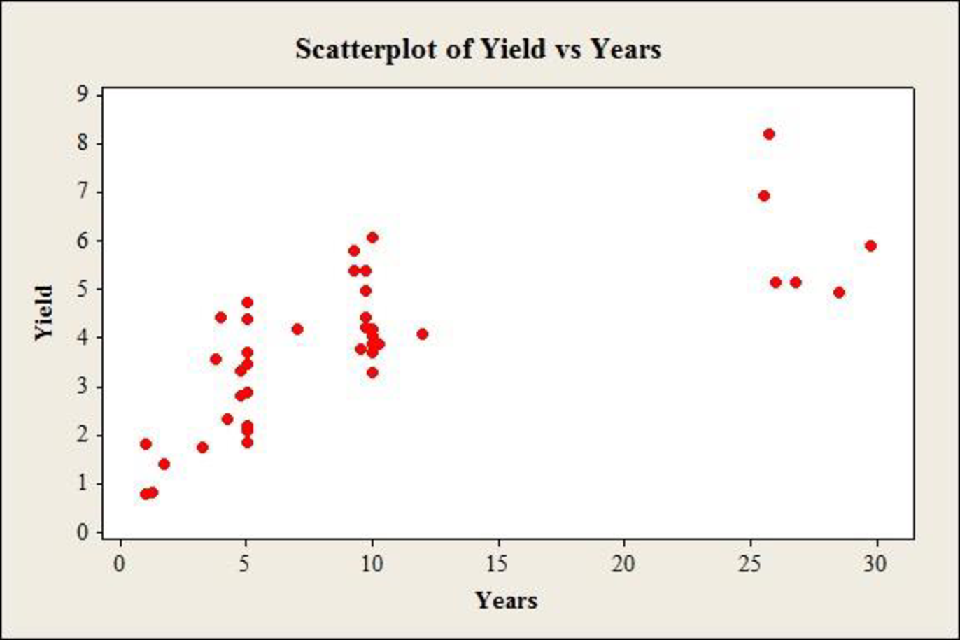
A simple linear regression model does not appear to be appropriate.
Explanation of Solution
Calculation:
The data gives information on yield (%) of 40 corporate bonds and the respective years to maturity.
Scatterplot:
Software procedure:
Step by step procedure to draw scatter diagram using MINITAB software is given below:
- Choose Graph > Scatterplot.
- Choose Simple, and then click OK.
- In Y–variables, enter the column of Yield.
- In X–variables enter the column of Years.
- Click OK.
Observation:
The scatterplot shows a gradual increase in the yield, at a decreasing rate, with increase in years up to 25. After this, there is a reduction in the values of yield. Thus, a simple linear regression model does not appear to be appropriate.
b.
Develop an estimated multiple regression equation with
Answer to Problem 29SE
The estimated multiple regression equation with
Explanation of Solution
Calculation:
Square transformation:
Software procedure:
Step by step procedure to make square transformation using MINITAB software is given as,
- Choose Calc > Calculator.
- In Store result in variable, enter YearsSq.
- In Expression, enter ‘Years’^2.
- Click OK.
The squared variable is stored in the column of ‘YearsSq’.
Regression:
Software procedure:
Step by step procedure to obtain the regression equation using MINITAB software:
- Choose Stat > Regression > General Regression.
- Under Responses, enter the column of Yield.
- Under Model, enter the columns of Years, YearsSq.
- Click OK.
Output using MINITAB software is given below:
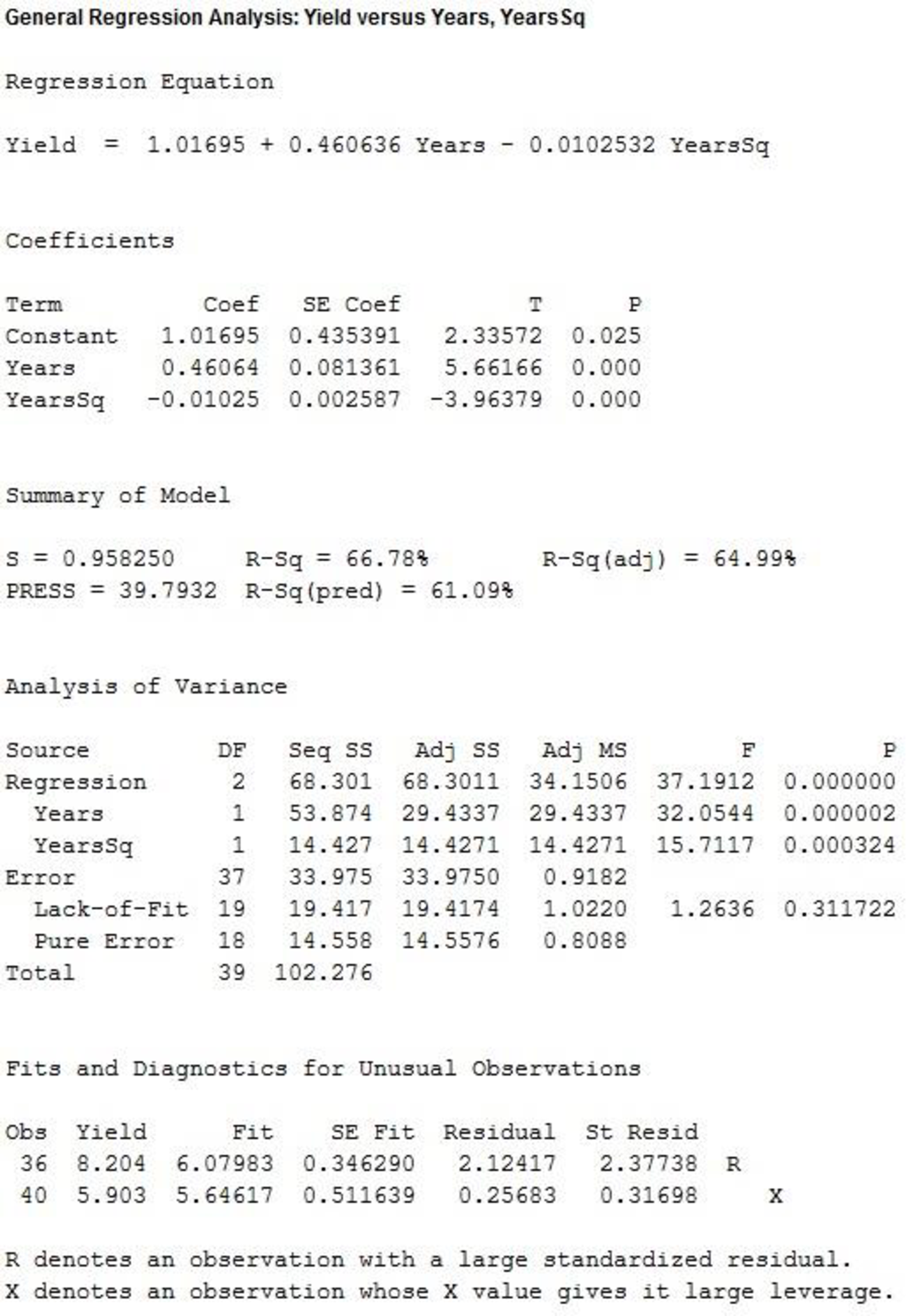
From the output, the estimated multiple regression equation with
c.
Develop an estimated multiple regression equation using the natural logarithm of years as the independent variable.
Explain whether the current regression provides a better fit than the estimated regression developed in part b.
Answer to Problem 29SE
The estimated multiple regression equation using the natural logarithm of years as the independent variable is:
The estimated regression using the natural logarithm of x provides a better fit than the estimated regression developed in part b.
Explanation of Solution
Calculation:
Logarithmic transformation:
Software procedure:
Step by step procedure to make logarithmic transformation using MINITAB software is given as,
- Choose Calc > Calculator.
- In Store result in variable, enter Years.
- In Expression, enter ln(‘Years’).
- Click OK.
The logarithm of the variable is stored in the column of ‘ln(‘Years’)’.
Regression:
Software procedure:
Step by step procedure to obtain the regression equation using MINITAB software:
- Choose Stat > Regression > General Regression.
- Under Responses, enter the column of Yield.
- Under Model, enter the columns of ln(Years).
- Click OK.
Output using MINITAB software is given below:
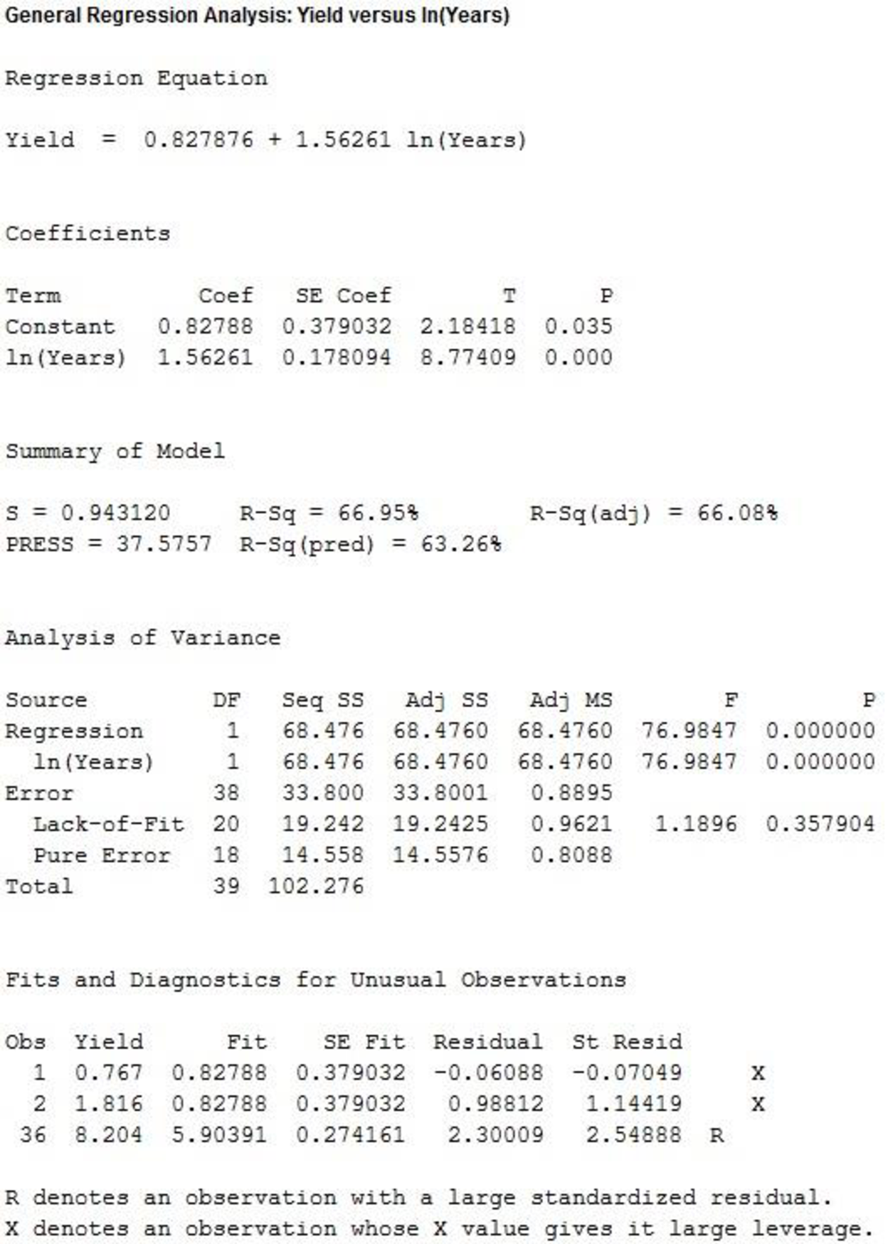
From the output, the estimated multiple regression equation using the natural logarithm of years as the independent variable is:
Adjusted-
The adjusted
The value of adjusted
The value of adjusted
Evidently, the current regression equation effectively explains more of the variation the response variable, than the second regression equation.
Thus, the estimated regression using the natural logarithm of x provides a better fit than the estimated regression developed in part b.
Want to see more full solutions like this?
Chapter 16 Solutions
Statistics for Business & Economics


- Olympic Pole Vault The graph in Figure 7 indicates that in recent years the winning Olympic men’s pole vault height has fallen below the value predicted by the regression line in Example 2. This might have occurred because when the pole vault was a new event there was much room for improvement in vaulters’ performances, whereas now even the best training can produce only incremental advances. Let’s see whether concentrating on more recent results gives a better predictor of future records. (a) Use the data in Table 2 (page 176) to complete the table of winning pole vault heights shown in the margin. (Note that we are using x=0 to correspond to the year 1972, where this restricted data set begins.) (b) Find the regression line for the data in part ‚(a). (c) Plot the data and the regression line on the same axes. Does the regression line seem to provide a good model for the data? (d) What does the regression line predict as the winning pole vault height for the 2012 Olympics? Compare this predicted value to the actual 2012 winning height of 5.97 m, as described on page 177. Has this new regression line provided a better prediction than the line in Example 2?arrow_forwardDoes the sugar cane model suffer from heteroscedasticity? Perform a Breusch-Pegan test as well as a Whitetest to verify what the residual plots suggests, based on the following regression results:arrow_forwardThe operations manager of a musical instrument distributor feels that the demand for Bass Drums may be related to the number of television appearances by the popular rick group Green Shades during the previous month. The manager has collected the data shown in the following table. Demand for Bass Drums 3 6 7 5 10 8 Green Shades TV appearances 3 4 7 6 8 5 Develop the linear regression equation to forecast. Forecast demand for Bass Drums when Green Shades’ TV appearances are 10. Compute MSE and standard deviation for Problem 8.arrow_forward
- The Update to the Task Force Report on Blood Pressure Control in Children [12] reported the observed 90th per-centile of SBP in single years of age from age 1 to 17 based on prior studies. The data for boys of average height are given in Table 11.18. Suppose we seek a more efficient way to display the data and choose linear regression to accomplish this task. age sbp 1 99 2 102 3 105 4 107 5 108 6 110 7 111 8 112 9 114 10 115 11 117 12 120 13 122 14 125 15 127 16 130 17 132 Do you think the linear regression provides a good fit to the data? Why or why not? Use residual analysis to justify your answer. Am I supposed to run a residual plot and QQ-plot for this question?arrow_forwardIf the point representing 64 wins and attendance of 40,786, people per game is removed from the set of data and a new regression analysis is conducted, how would the following be mpacted?arrow_forwardIf there is no significant correlation between the response and explanatory variables, would the slope of the regression line be (a) positive (b) negative (c) zero?arrow_forward
- A mail-order business selling personal computer supplies, software and hardware maintains a centralized warehouse. Management is currently examining the process of distribution from the warehouse and wants to study the factors that affect the warehouse distribution costs. Data collected over 24 random months contain the warehouse’s distribution cost (in thousands of Rands), the sales (in thousands of Rands) and the number of orders received. A multiple linear regression model was fitted to the data by using Stat1.2. Use the output to answer the questions that follow by typing only the letter of the correct option in the answer boxes. Variablesy: Warehouse Distribution Costx1: Salesx2: Number of Orders Model Fitting StatisticsR2 = 0.8504Adj R2: ? Regression Coefficients Beta Parameter Standard b Parameter Standard Estimates…arrow_forwardTo evaluate whether the assumption of linearity has been violated, which of the following graph should be examined? A. QQ plot of residuals B. Predicted Values vs. Residuals C. Residuals vs. Progrm Per-Year Tuition ($) D. Residual index plot b) To evaluate whether the assumption of normality has been violated, which of the following graph should be examined? A. Predicted Values vs. Residuals B. Residuals vs. Progrm Per-Year Tuition ($) C. Residual index plot D. QQ plot of residuals c) To evaluate whether the assumption of equal variance has been violated, which of the following graph should be examined? A. Predicted Values vs. Residuals B. Residual index plot C. Residuals vs. Progrm Per-Year Tuition ($) D. QQ plot of residuals d) To evaluate whether the assumption of independence has been violated, which of the folowing graph should be examined? A. Residual index plot…arrow_forwardThe personnel director of a large hospital is interested in determining the relationship (if any) between an employee’s age and the number of sick days the employee takes per year. The director randomly selects ten employees and records their age and the number of sick days which they took in the previous year. Employee 1 2 3 4 5 6 7 8 9 10Age 30 50 40 55 30 28 60 25 30 45Sick Days 7 4 3 2 9 10 0 8 5 2 The estimated regression equation and the standard error are given. Sick Days=14.310162−0.236900(Age) Se=1.682207 Find the 95% prediction interval for the average number of sick days an employee will take per year, given the employee is 34 . Round your answer to two decimal places.arrow_forward
 College AlgebraAlgebraISBN:9781305115545Author:James Stewart, Lothar Redlin, Saleem WatsonPublisher:Cengage Learning
 Linear Algebra: A Modern IntroductionAlgebraISBN:9781285463247Author:David PoolePublisher:Cengage Learning
 Glencoe Algebra 1, Student Edition, 9780079039897...AlgebraISBN:9780079039897Author:CarterPublisher:McGraw Hill