STATISTICS F/BUSINESS+ECONOMICS-TEXT
13th Edition
ISBN: 9781305881884
Author: Anderson
Publisher: CENGAGE L
expand_more
expand_more
format_list_bulleted
Videos
Textbook Question
Chapter 17.6, Problem 38E
Three years of monthly lawn-maintenance expenses ($) for a six-unit apartment house in southern Florida follow.
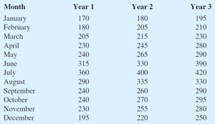
- a. Construct a time series plot. What type of pattern exists in the data?
- b. Identify the monthly seasonal indexes for the three years of lawn-maintenance expenses for the apartment house in southern Florida as given here. Use a 12-month moving average calculation.
- c. Deseasonalize the time series.
- d. Compute the linear trend equation for the deseasonalized data.
- e. Compute the deseasonalized trend forecasts and then adjust the trend forecasts using the seasonal indexes to provide a forecast for monthly expenses in year 4.
Expert Solution & Answer
Want to see the full answer?
Check out a sample textbook solution
Students have asked these similar questions
the values of alabama building contracts (in $ millions) for a 12-month period follow.240 350 230 260 280 320 220 310 240 310 240 230a. construct a time series plot. What type of pattern exists in the data?
Year Gross Federal Debt ($millions)
1945 260,123
1950 256,853
1955 274,366
1960 290,525
1965 322,318
1970 380,921
1975 541,925
1980 909,050
1985 1,817,521
1990 3,206,564
1995 4,921,005
2000 5,686,338
Construct a scatter plot with this data. Do you observe a trend? If so, what type of trend do you observe?
Use Excel to fit a linear trend and an exponential trend to the data. Display the models and their respective r^2.
Interpret both models. Which model seems to be more appropriate? Why?
Which of the following time series forecasting methods would not be used to forecast seasonal data?
Chapter 17 Solutions
STATISTICS F/BUSINESS+ECONOMICS-TEXT
Ch. 17.2 - Consider the following time series data. Week 1 2...Ch. 17.2 - Refer to the time series data in exercise 1. Using...Ch. 17.2 - Exercises 1 and 2 used different forecasting...Ch. 17.2 - Consider the following time series data. Month 1 2...Ch. 17.3 - Consider the following time series data. Week 1 2...Ch. 17.3 - Consider the following time series data. Month 1 2...Ch. 17.3 - Refer to the gasoline sales time series data in...Ch. 17.3 - Refer again to the gasoline sales time series data...Ch. 17.3 - With the gasoline time series data from Table...Ch. 17.3 - With a smoothing constant of = .2, equation...
Ch. 17.3 - For the Hawkins Company, the monthly percentages...Ch. 17.3 - Corporate triple-A bond interest rates for 12...Ch. 17.3 - The values of Alabama building contracts (in ...Ch. 17.3 - The following time series shows the sales of a...Ch. 17.3 - Ten weeks of data on the Commodity Futures Index...Ch. 17.3 - The U.S. Census Bureau tracks the median price for...Ch. 17.4 - Consider the following time series data. a....Ch. 17.4 - Prob. 18ECh. 17.4 - Consider the following time series. a. Construct a...Ch. 17.4 - Prob. 20ECh. 17.4 - Prob. 21ECh. 17.4 - The Seneca Childrens Fund (SCF) is a local charity...Ch. 17.4 - The following table shows Googles annual revenue...Ch. 17.4 - FRED (Federal Reserve Economic Data), a database...Ch. 17.4 - Quarterly revenue ( millions) for Twitter for the...Ch. 17.4 - Giovanni Food Products produces and sells frozen...Ch. 17.4 - Prob. 27ECh. 17.5 - Consider the following time series. a. Construct a...Ch. 17.5 - Consider the following time series data. a....Ch. 17.5 - The quarterly sales data (number of copies sold)...Ch. 17.5 - Air pollution control specialists in southern...Ch. 17.5 - South Shore Construction builds permanent docks...Ch. 17.5 - Prob. 33ECh. 17.5 - Three years of monthly lawn-maintenance expenses...Ch. 17.6 - Consider the following time series data. a....Ch. 17.6 - Refer to exercise 35. a. Deseasonalize the time...Ch. 17.6 - The quarterly sales data (number of copies sold)...Ch. 17.6 - Three years of monthly lawn-maintenance expenses...Ch. 17.6 - Air pollution control specialists in southern...Ch. 17.6 - Electric power consumption is measured in...Ch. 17 - The weekly demand (in cases) for a particular...Ch. 17 - The following table reports the percentage of...Ch. 17 - United Dairies. Inc., supplies milk to several...Ch. 17 - The data contained in the DATAfile named CrudeCost...Ch. 17 - Annual retail store revenue for Apple from 2007 to...Ch. 17 - The Mayfair Department Store in Davenport, Iowa,...Ch. 17 - Prob. 47SECh. 17 - The Costello Music Company has been in business...Ch. 17 - Consider the Costello Music Company problem in...Ch. 17 - Refer to the Costello Music Company problem in...Ch. 17 - Refer to the Costello Music Company time series in...Ch. 17 - Hudson Marine has been an authorized dealer for CD...Ch. 17 - Refer to the Hudson Marine problem in exercise 52....Ch. 17 - Refer to the Hudson Marine problem in exercise 53....Ch. 17 - Refer to the Hudson Marine data in exercise 53. a....Ch. 17 - Forecasting Food and Beverage Sales The Vintage...Ch. 17 - Forecasting Lost Sales The Carlson Department...
Knowledge Booster


Learn more about
Need a deep-dive on the concept behind this application? Look no further. Learn more about this topic, statistics and related others by exploring similar questions and additional content below.Similar questions
- After its move in 1990 to La Junta, Colorado, and its new initiatives, the DeBourgh Manufacturing Company began an upward climb of record sales. Suppose the figures shown here are the DeBourgh monthly sales figures from January 2001 through December 2009 (in $1,000s). a) Produce a time series plot. Are there any trends evident in the data? Does DeBourgh have a seasonal component to its sales? b) Deseasonalize the data using Multiplicative model with a 0.5 weighted moving average. Produce a time series plot of the deseasonalized data and add a trendline. c) Forecast the sales from January to December of the year 2010. d) Include a discussion of the general direction of sales and any seasonal tendencies that might be occurrinG Month 2001 2002 2003 2004 2005 2006 2007 2008 2009 January 139.7 165.1 177.8 228.6 266.7 431.8 381 431.8 495.3 February 114.3 177.8 203.2 254 317.5 457.2 406.4 444.5 533.4 March 101.6 177.8 228.6 266.7 368.3 457.2 431.8 495.3 635 April 152.4 203.2…arrow_forwardDescribe the following time-series patterns: a. Horizontal Pattern b. Trend Pattern c. Seasonal Pattern d. Cyclical Patternarrow_forwardFor the hawkins company, the monthly percentages of all shipments received on timeover the past 12 months are 80, 82, 84, 83, 83, 84, 85, 84, 82, 83, 84, and 83.a. construct a time series plot. What type of pattern exists in the data?arrow_forward
- The president of State University wants to forecast student enrollments for this Year academic year based on the following historical data: 5 years ago 4 years ago 3 years ago 2 years ago Last year Enrollments 15.000 16.000 18.000 20.000 21.000 a- What is the forecast for this year using a 3-year weighted moving average where the weights are halved in a descending order from newest to oldest ? b. What is the forecast for this year using the trend line for these data? c. using the MAD find which forecasting technique may be appropriate for this quetionarrow_forwardThe following data set provides the total number of shipments of core major household appliances in the U.S. from 2000 to 2016 (in millions): Year Shipments (millions) 2000 38.4 2001 38.2 2002 40.8 2003 42.5 2004 46.1 2005 47.0 2006 46.7 2007 44.1 2008 39.8 2009 36.5 2010 38.2 2011 36.0 2012 35.8 2013 39.2 2014 41.5 2015 42.9 2016 44.7 a. Plot the time series. b. Fit a three-year moving average to the data and plot the results. c. Fit a five-year moving average to the data and plot the results. d. Compute a linear trend forecasting equation and plot the trend line. e. Compute a quadratic trend forecasting equation and plot the results.arrow_forwardThe report “Daily Cigarette Use: Indicators on Children and Youth" (Child Trends Data Bank, childtrends.org/wp-content/uploads/2012/11/03 _Smoking_new.pdf, retrieved April 17, 2017) included the accompanying data on the percentage of students who report smoking cigarettes daily, for students in grades 8, 10, and 12. Construct a time series plot for students in grade 12, and comment on any trend over time. Construct a time series plot that shows trends over time for each of the three grade levels. Graph each of the three-time series on the same set of axes, using different colors to distinguish the different grade levels. Either label the time series in the plot or include a legend to indicate which time series corresponds to which grade level. Write a paragraph based on the plot from Part (b). Discuss the similarities and differences for the three grade levelsarrow_forward
- Consider the following time seriesweek 1 2 3 4 5 6 value 18 13 16 11 17 14 a) Construct a time series plot? What type of pattern exists in the datab) Develop the three week moving average forecasts for this time series, then compute the measures of forecasts accurecyarrow_forwardUse quantitativeforecast methods for the data shown below Period Observation 1 24 2 34 3 36 4 37 5 41 6 44 7 45 Plot the original time series and comment on appropriateness of a linear trend.arrow_forwardWhich of the time series forecasting methods would not be used to forecast seasonal data?arrow_forward
- Find out the next month after april income by using the forecasting method of the moving average methodarrow_forwardIllustrate the formulation of dynamic causal effects in time series data?arrow_forwardThe table below contains the average price paid for a new home in a certain area from 2000 to 2010. a. Construct a time-series plot of new home prices. b. What pattern, if any, is present in the data? Year Average_Price_($_thousands)2000 351.12001 330.52002 310.52003 296.72004 229.72005 182.32006 154.52007 156.32008 154.72009 154.52010 154.5arrow_forward
arrow_back_ios
SEE MORE QUESTIONS
arrow_forward_ios
Recommended textbooks for you
 MATLAB: An Introduction with ApplicationsStatisticsISBN:9781119256830Author:Amos GilatPublisher:John Wiley & Sons Inc
 Probability and Statistics for Engineering and th...StatisticsISBN:9781305251809Author:Jay L. DevorePublisher:Cengage Learning
 Statistics for The Behavioral Sciences (MindTap C...StatisticsISBN:9781305504912Author:Frederick J Gravetter, Larry B. WallnauPublisher:Cengage Learning
 Elementary Statistics: Picturing the World (7th E...StatisticsISBN:9780134683416Author:Ron Larson, Betsy FarberPublisher:PEARSON
 The Basic Practice of StatisticsStatisticsISBN:9781319042578Author:David S. Moore, William I. Notz, Michael A. FlignerPublisher:W. H. Freeman
 Introduction to the Practice of StatisticsStatisticsISBN:9781319013387Author:David S. Moore, George P. McCabe, Bruce A. CraigPublisher:W. H. Freeman
MATLAB: An Introduction with Applications
Statistics
ISBN:9781119256830
Author:Amos Gilat
Publisher:John Wiley & Sons Inc
Probability and Statistics for Engineering and th...
Statistics
ISBN:9781305251809
Author:Jay L. Devore
Publisher:Cengage Learning
Statistics for The Behavioral Sciences (MindTap C...
Statistics
ISBN:9781305504912
Author:Frederick J Gravetter, Larry B. Wallnau
Publisher:Cengage Learning
Elementary Statistics: Picturing the World (7th E...
Statistics
ISBN:9780134683416
Author:Ron Larson, Betsy Farber
Publisher:PEARSON
The Basic Practice of Statistics
Statistics
ISBN:9781319042578
Author:David S. Moore, William I. Notz, Michael A. Fligner
Publisher:W. H. Freeman
Introduction to the Practice of Statistics
Statistics
ISBN:9781319013387
Author:David S. Moore, George P. McCabe, Bruce A. Craig
Publisher:W. H. Freeman
Time Series Analysis Theory & Uni-variate Forecasting Techniques; Author: Analytics University;https://www.youtube.com/watch?v=_X5q9FYLGxM;License: Standard YouTube License, CC-BY
Operations management 101: Time-series, forecasting introduction; Author: Brandoz Foltz;https://www.youtube.com/watch?v=EaqZP36ool8;License: Standard YouTube License, CC-BY