
Concept explainers
Videos
a.
Construct the frequency distribution with a class width of 5 and a lower limit of 45 for the first class.
a.
Answer to Problem 10RE
The frequency distribution is,
| Age | Frequency |
| 45-49 | 2 |
| 50-54 | 1 |
| 55-59 | 4 |
| 60-64 | 6 |
| 65-69 | 6 |
| 70-74 | 6 |
| 75-79 | 4 |
| 80-84 | 3 |
| 85-89 | 2 |
| 90-94 | 4 |
| Total | 38 |
Explanation of Solution
Calculation:
The given information is that a data representing the age at which the all U.S. presidents died.
Frequency:
The frequencies are calculated by using the tally mark and the
- Based on the given information, the class intervals are 45-49, 50-54, 55-59, 60-64, 65-69, 70-74, 75-79, 80-84, 85-89, 90-94.
- Make a tally mark for each value in the corresponding age class and continue for all values in the data.
- The number of tally marks in each class represents the frequency, f of that class.
Similarly, the frequency of remaining classes for the age is given below:
| Age | Tally | Frequency |
| 45-49 | 2 | |
| 50-54 | 1 | |
| 55-59 | 4 | |
| 60-64 | 6 | |
| 65-69 | 6 | |
| 70-74 | 6 | |
| 75-79 | 4 | |
| 80-84 | 3 | |
| 85-89 | 2 | |
| 90-94 | 4 | |
| Total | 38 |
b.
Construct the frequency histogram based on the frequency distribution.
b.
Answer to Problem 10RE
Output obtained from MINITAB software for the ages is:
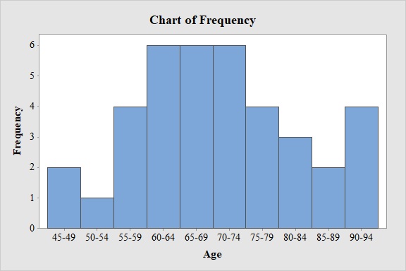
Explanation of Solution
Calculation:
Frequency Histogram:
Software procedure:
- Step by step procedure to draw the frequency histogram for the ages using MINITAB software.
- Choose Graph > Bar Chart.
- From Bars represent, choose unique values from table.
- Choose Simple.
- Click OK.
- In Graph variables, enter the column of Frequency.
- In Categorical variables, enter the column of Ages.
- Click OK
- Select Edit Scale, Enter 0 in Gap between clusters.
Observation:
From the bar graph, it can be seen that maximum age at death for the U.S. presidents is in the interval 60-75.
c.
Construct a relative frequency distribution for the data.
c.
Answer to Problem 10RE
The relative frequency distribution for the data is:
| Age | Relative frequency |
| 45-49 | 0.053 |
| 50-54 | 0.026 |
| 55-59 | 0.105 |
| 60-64 | 0.158 |
| 65-69 | 0.158 |
| 70-74 | 0.158 |
| 75-79 | 0.105 |
| 80-84 | 0.079 |
| 85-89 | 0.053 |
| 90-94 | 0.105 |
Explanation of Solution
Calculation:
Relative frequency:
The general formula for the relative frequency is,
Therefore,
Similarly, the relative frequencies for the remaining ages are obtained below:
| Age | Frequency | Relative frequency |
| 45-49 | 2 | |
| 50-54 | 1 | |
| 55-59 | 4 | |
| 60-64 | 6 | |
| 65-69 | 6 | |
| 70-74 | 6 | |
| 75-79 | 4 | |
| 80-84 | 3 | |
| 85-89 | 2 | |
| 90-94 | 4 | |
| Total | 38 |
d.
Construct the relative frequency histogram based on the frequency distribution.
d.
Answer to Problem 10RE
Output obtained from MINITAB software for the ages is:
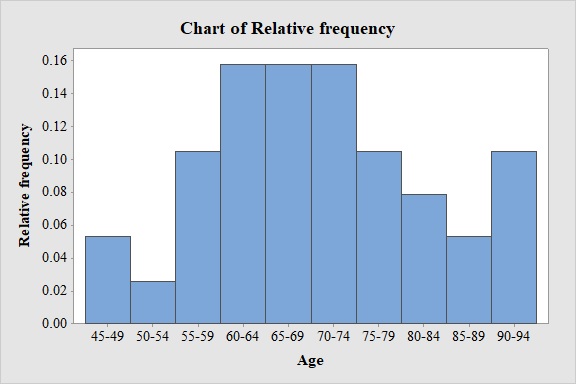
Explanation of Solution
Calculation:
Relative Frequency Histogram:
Software procedure:
- Step by step procedure to draw the relative frequency histogram for the ages using MINITAB software.
- Choose Graph > Bar Chart.
- From Bars represent, choose unique values from table.
- Choose Simple.
- Click OK.
- In Graph variables, enter the column of Relative Frequency.
- In Categorical variables, enter the column of Ages.
- Click OK
- Select Edit Scale, Enter 0 in Gap between clusters.
Observation:
From the bar graph, it can be seen that maximum age at death for the U.S. presidents is in the interval 60-75.
Want to see more full solutions like this?
Chapter 2 Solutions
Essential Statistics


 MATLAB: An Introduction with ApplicationsStatisticsISBN:9781119256830Author:Amos GilatPublisher:John Wiley & Sons Inc
 Probability and Statistics for Engineering and th...StatisticsISBN:9781305251809Author:Jay L. DevorePublisher:Cengage Learning
 Statistics for The Behavioral Sciences (MindTap C...StatisticsISBN:9781305504912Author:Frederick J Gravetter, Larry B. WallnauPublisher:Cengage Learning
 Elementary Statistics: Picturing the World (7th E...StatisticsISBN:9780134683416Author:Ron Larson, Betsy FarberPublisher:PEARSON
 The Basic Practice of StatisticsStatisticsISBN:9781319042578Author:David S. Moore, William I. Notz, Michael A. FlignerPublisher:W. H. Freeman
 Introduction to the Practice of StatisticsStatisticsISBN:9781319013387Author:David S. Moore, George P. McCabe, Bruce A. CraigPublisher:W. H. Freeman