Chapter 2, Problem 6RE

a.

To determine

Find the number of classes.

Answer to Problem 6RE

The number of classes is 8.

Explanation of Solution

The given information is a frequency distribution corresponding to the number of freshmen elected in each of the elections.

From the frequency distribution, it can be observed that there are 8 classes.

Thus, the number of classes is 8.

b.

To determine

Find the class width of the given frequency distribution.

Answer to Problem 6RE

The class width of the data is 20.

Explanation of Solution

Calculation:

The class width is determined by the formula as follows:

$\text{Class}\text{width}\text{=Lower}\text{limit for the second class-}\text{Lower}\text{limitfor the first class}$

Substitute 40 as “Lower limit for the second class” and 20 as “Lower limit for the first class”.

$\begin{array}{c}\text{Class}\text{width}\text{=}40-\text{20}\\ \text{=20}\end{array}$

For each class “Class width” is same.

Thus, the class width is 20.

c.

To determine

List the class limits.

Answer to Problem 6RE

The lower class limits are 20, 40, 60, 80, 100, 120, 140, 160 and the upper class limits are 39, 59, 79, 99, 119, 139, 159, 179.

Explanation of Solution

Lower class limits:

The smallest value that is appear in a class interval is called lower class limits for that class.

Upper class limits:

The largest value that is appear in a class interval is called upper class limits for that class.

From the frequency distribution, it can be observed that there are 8 classes. The smallest and largest values in the class 20-39 are 20 and 39. Thus, the lower class limit for the class 20-39 is 20 and upper class limit is 39.

Similarly the remaining lower class limits are 20, 40, 60, 80, 100, 120, 140, 160 and the upper class limits are 39, 59, 79, 99, 119, 139, 159, 179.

Thus, the lower and upper class limits are 20, 40, 60, 80, 100, 120, 140, 160 and 339, 59, 79, 99, 119, 139, 159, 179 respectively.

d.

To determine

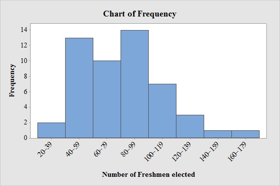
Construct a frequency histogram.

Answer to Problem 6RE

Output obtained from MINITAB software for number of freshmen elected is:

Explanation of Solution

Calculation:

Software procedure:

• Step by step procedure to draw the frequency histogram for number of freshmen elected using MINITAB software.
• Choose Graph > Bar Chart.
• From Bars represent, choose unique values from table.
• Choose Simple.
• Click OK.
• In Graph variables, enter the column of Frequency.
• In Categorical variables, enter the column of Number of Freshmen elected.
• Click OK
• Select Edit Scale, Enter 0 in Gap between clusters.

Observation:

From the bar graph, it can be seen that the maximum number of freshmen elected is in the class interval 80-99.

e.

To determine

Construct a relative frequency distribution for the data.

Answer to Problem 6RE

The relative frequency distribution for the data is:

Number of Freshmen elected	Relative Frequency
20-39	0.039
40-59	0.255
60-79	0.196
80-99	0.275
100-119	0.137
120-139	0.059
140-159	0.020
160-179	0.020

Explanation of Solution

Calculation:

Relative frequency:

The general formula for the relative frequency is,

$\text{Relative}\text{Frequency = }\frac{\text{Frequency}}{\text{Total frequency}}$

Therefore,

$\begin{array}{c}\text{Relative}\text{Frequency}\text{for the class 20-39}=\frac{2}{51}\\ =0.039\end{array}$

Similarly, the relative frequencies for number of freshmen elected are obtained below:

Number of Freshmen elected	Frequency	Relative Frequency
20-39	2	$\frac{2}{51}=0.039$
40-59	13	$\frac{13}{51}=0.255$
60-79	10	$\frac{10}{51}=0.196$
80-99	14	$\frac{14}{51}=0.275$
100-119	7	$\frac{7}{51}=0.137$
120-139	3	$\frac{3}{51}=0.059$
140-159	1	$\frac{1}{51}=0.020$
160-179	1	$\frac{1}{51}=0.020$

f.

To determine

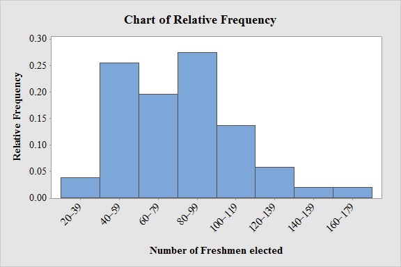
Construct a relative frequency histogram for these data.

Answer to Problem 6RE

Output obtained from MINITAB software for number of freshmen elected is:

Explanation of Solution

Calculation:

Relative Frequency Histogram:

Software procedure:

• Step by step procedure to draw the relative frequency histogram for number of freshmen elected using MINITAB software.
• Choose Graph > Bar Chart.
• From Bars represent, choose unique values from table.
• Choose Simple.
• Click OK.
• In Graph variables, enter the column of Relative Frequency.
• In Categorical variables, enter the column of Number of Freshmen elected.
• Click OK
• Select Edit Scale, Enter 0 in Gap between clusters.

Observation:

From the bar graph, it can be seen that the maximum number of freshmen elected is in the class interval 80-99.