
Videos
BMW prices: The following table presents the manufacturer’s suggested retail price (in $1000s) for recent base models and styles of BMW automobiles.
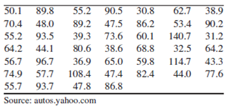
- a. Construct a frequency distribution using a class width of 10, and using 30 as the lower class limit for the first class.
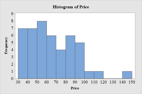
- b. Construct a frequency histogram from the frequency distribution in part (a).
- c. Construct a relative frequency distribution using the same class width and lower limit for the first class.
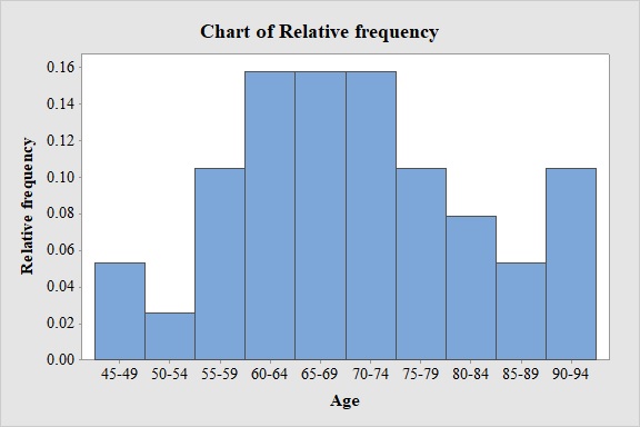
- d. Construct a relative frequency histogram.
- e. Are the histograms unimodal or bimodal?
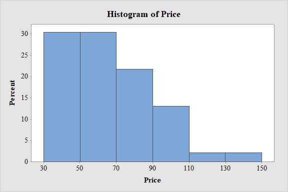
- f. Repeat parts (a)–(d), using a class width of 20, and using 30 as the lower class limit for the first class.
- g. Do you think that class widths of 10 and 20 are both reasonably good choices for these data, or do you think that one choice is much better than the other? Explain your reasoning.
a.
Construct the frequency distribution with a class width of 10 and a lower limit of 30 for the first class.
Answer to Problem 29E
The frequency distribution is,
| Price($1000s) | Frequency |
| 30-39.9 | 7 |
| 40-49.9 | 7 |
| 50-59.9 | 8 |
| 60-69.9 | 6 |
| 70-79.9 | 4 |
| 80-89.9 | 6 |
| 90-99.9 | 5 |
| 100-109.9 | 1 |
| 110-119.9 | 1 |
| 120-129.9 | 0 |
| 130-139.9 | 0 |
| 140-149.9 | 1 |
| Total | 46 |
Explanation of Solution
Calculation:
The given information is that a table representing the manufacturer’s suggested retail price (in $1000s) for recent base models and style of BMW automobiles.
Frequency:
The frequencies are calculated by using the tally mark and the range of the data is from 30 to 149.9.
- Based on the given information, the class intervals are 30-39.9, 40-49.9, 50-59.9, 60-69.9, 70-79.9, 80-89.9, 90-99.9, 100-109.9, 110-119.9, 120-129.9, 130-139.9, 140-149.9.
- Make a tally mark for each value in the corresponding price class and continue for all values in the data.
- The number of tally marks in each class represents the frequency, f of that class.
Similarly, the frequency of remaining classes for the price is given below:
| Price($1000s) | Tally | Frequency |
| 30-39.9 | 7 | |
| 40-49.9 | 7 | |
| 50-59.9 | 8 | |
| 60-69.9 | 6 | |
| 70-79.9 | 4 | |
| 80-89.9 | 6 | |
| 90-99.9 | 5 | |
| 100-109.9 | 1 | |
| 110-119.9 | 1 | |
| 120-129.9 | 0 | |
| 130-139.9 | 0 | |
| 140-149.9 | 1 | |
| Total | 46 |
b.
Construct the frequency histogram based on the frequency distribution.
Answer to Problem 29E
Output obtained from MINITAB software for the price is:
Explanation of Solution
Calculation:
Frequency Histogram:
Software procedure:
- Step by step procedure to draw the relative frequency histogram for price using MINITAB software.
- Choose Graph > Histogram.
- Choose Simple.
- Click OK.
- In Graph variables, enter the column of Price.
- In Scale, Choose Y-scale Type as Frequency.
- Click OK.
- Select Edit Scale, Enter 30,40,50,60,70,80,90,100,110,120,130,140 in Positions of ticks.
- In Binning, Under Interval Type select Cutpoint and under Interval Definition select Number of intervals as 12 and Cutpoint positions as 30,40,50,60,70,80,90,100,110,120,130,140.
- In Labels, Enter 30,40,50,60,70,80,90,100,110,120,130,140 in Specified.
- Click OK.
Observation:
From the bar graph, it can be seen that maximum retail price is in the interval 50-60.
c.
Construct a relative frequency distribution for the data.
Answer to Problem 29E
The relative frequency distribution for the data is:
| Price($1000s) | Relative frequency |
| 30-39.9 | 0.152 |
| 40-49.9 | 0.152 |
| 50-59.9 | 0.174 |
| 60-69.9 | 0.130 |
| 70-79.9 | 0.087 |
| 80-89.9 | 0.130 |
| 90-99.9 | 0.109 |
| 100-109.9 | 0.022 |
| 110-119.9 | 0.022 |
| 120-129.9 | 0.000 |
| 130-139.9 | 0.000 |
| 140-149.9 | 0.022 |
Explanation of Solution
Calculation:
Relative frequency:
The general formula for the relative frequency is,
Therefore,
Similarly, the relative frequencies for the remaining prices are obtained below:
| Price($1000s) | Frequency | Relative frequency |
| 30-39.9 | 7 | |
| 40-49.9 | 7 | |
| 50-59.9 | 8 | |
| 60-69.9 | 6 | |
| 70-79.9 | 4 | |
| 80-89.9 | 6 | |
| 90-99.9 | 5 | |
| 100-109.9 | 1 | |
| 110-119.9 | 1 | |
| 120-129.9 | 0 | |
| 130-139.9 | 0 | |
| 140-149.9 | 1 | |
| Total | 46 |
d.
Construct the relative frequency histogram based on the frequency distribution.
Answer to Problem 29E
Output obtained from MINITAB software for the price is:
Explanation of Solution
Calculation:
Relative Frequency Histogram:
Software procedure:
- Step by step procedure to draw the relative frequency histogram for the price using MINITAB software.
- Choose Graph > Histogram.
- Choose Simple.
- Click OK.
- In Graph variables, enter the column of 'Mileage for 2000 cars'.
- In Scale, Choose Y-scale Type as Percent.
- Click OK.
- Select Edit Scale, Enter 30,40,50,60,70,80,90,100,110,120,130,140 in Positions of ticks.
- In Binning, Under Interval Type select Cutpoint and under Interval Definition select Number of intervals as 12 and Cutpoint positions as 30,40,50,60,70,80,90,100,110,120,130,140.
- In Labels, Enter 30,40,50,60,70,80,90,100,110,120,130,140 in Specified.
- Click OK.
Observation:
From the bar graph, it can be seen that maximum retail price is in the interval 50-60.
e.
Check whether the histogram is unimodal or bimodal.
Answer to Problem 29E
The histogram is unimodal.
Explanation of Solution
From the given histogram, it can be observed that there is one most frequently occurring value in the data set. Thus, the distribution has only one mode.
Hence, the histogram is unimodal.
e.
Repeat parts (a) to (d), using a class width of 20 and a lower limit of 30 for the first class.
Answer to Problem 29E
The frequency distribution is,
| Price($1000s) | Frequency |
| 30-49.9 | 14 |
| 50-69.9 | 14 |
| 70-89.9 | 10 |
| 90-109.9 | 6 |
| 110-129.9 | 1 |
| 130-149.9 | 1 |
| Total | 46 |
Output obtained from MINITAB software for the price is:

The relative frequency distribution for the data is:
| Price($1000s) | Relative frequency |
| 30-39.9 | 0.304 |
| 50-59.9 | 0.304 |
| 70-79.9 | 0.217 |
| 90-99.9 | 0.130 |
| 110-119.9 | 0.022 |
| 130-139.9 | 0.022 |
Output obtained from MINITAB software for the price is:
Explanation of Solution
Calculation:
Frequency:
The frequencies are calculated by using the tally mark and the range of the data is from 30 to 149.9.
- Based on the given information, the class intervals are 30-49.9, 50-69.9, 70-89.9, 90-109.9, 110-129.9, 130-149.9.
- Make a tally mark for each value in the corresponding price class and continue for all values in the data.
- The number of tally marks in each class represents the frequency, f of that class.
Similarly, the frequency of remaining classes for the price is given below:
| Price($1000s) | Tally | Frequency |
| 30-49.9 | 14 | |
| 50-69.9 | 14 | |
| 70-89.9 | 10 | |
| 90-109.9 | 6 | |
| 110-129.9 | 1 | |
| 130-149.9 | 1 | |
| Total | 46 |
Frequency Histogram:
Software procedure:
- Step by step procedure to draw the relative frequency histogram for price using MINITAB software.
- Choose Graph > Histogram.
- Choose Simple.
- Click OK.
- In Graph variables, enter the column of Price.
- In Scale, Choose Y-scale Type as Frequency.
- Click OK.
- Select Edit Scale, Enter 30, 50, 70, 90, 110, 130 in Positions of ticks.
- In Binning, Under Interval Type select Cutpoint and under Interval Definition select Number of intervals as 12 and Cutpoint positions as 30, 50, 70, 90, 110, 130
- In Labels, Enter 30, 50, 70, 90, 110, 130 in Specified.
- Click OK.
Observation:
From the bar graph, it can be seen that maximum retail price is in the interval 30-70.
Relative frequency:
The general formula for the relative frequency is,
Therefore,
Similarly, the relative frequencies for the remaining prices are obtained below:
| Price($1000s) | Frequency | Relative frequency |
| 30-39.9 | 14 | |
| 50-59.9 | 14 | |
| 70-79.9 | 10 | |
| 90-99.9 | 6 | |
| 110-119.9 | 1 | |
| 130-139.9 | 1 | |
| Total | 46 |
Relative Frequency Histogram:
Software procedure:
- Step by step procedure to draw the relative frequency histogram for the price using MINITAB software.
- Choose Graph > Histogram.
- Choose Simple.
- Click OK.
- In Graph variables, enter the column of Price.
- In Scale, Choose Y-scale Type as Percent.
- Click OK.
- Select Edit Scale, Enter 30, 50, 70, 90, 110, 130 in Positions of ticks.
- In Binning, Under Interval Type select Cutpoint and under Interval Definition select Number of intervals as 12 and Cutpoint positions as 30, 50, 70, 90, 110, 130
- In Labels, Enter 30, 50, 70, 90, 110, 130 in Specified.
- Click OK.
Observation:
From the bar graph, it can be seen that maximum retail price is in the interval 30-70.
g.
Check whether the class widths of both 10 and 20 are reasonable or one choice is much better than the other and explain the reason.
Answer to Problem 29E
Both the class width of 10 and 20 are reasonable.
Explanation of Solution
Answer will vary.
The number of classes can be obtained by the following two points:
- The number of classes should be between 5 and 20.
- A larger number of classes will be appropriate for a very large data set.
Here number of classes for the histogram with class width 10 and 20 are 12 and 6 respectively. Thus, the number of classes should be between 5 and 20.
Hence, the class widths of both 10 and 20 are reasonable.
Want to see more full solutions like this?
Chapter 2 Solutions
Essential Statistics


 Glencoe Algebra 1, Student Edition, 9780079039897...AlgebraISBN:9780079039897Author:CarterPublisher:McGraw Hill