
Concept explainers
Videos
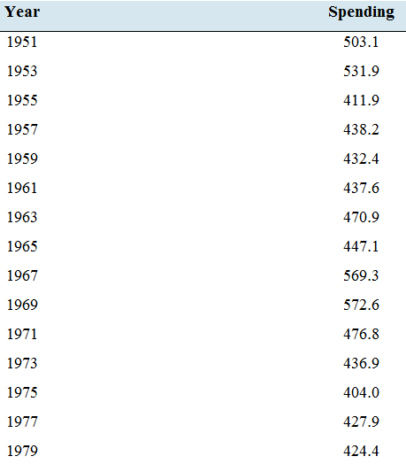
Military spending: The following table presents the amount spent, in billions of dollars, on national defense by the U.S. government every other year for the years 1951 through 2017. The amounts are adjusted for inflation, and represent 2017 dollars.
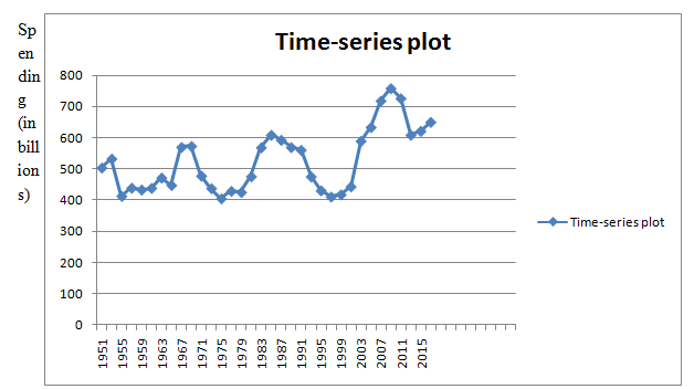
- Construct a time-series plot for these data.
- The plot covers seven decades, from the 1950s through the period 2010—2017. During which of these decades did national defense spending increase, and during which decades did it decrease?
- The United States fought in the Korean War, which ended in 1953. What effect did the end of the war have on military spending after 1953?
- During the period 1965—1963, the United States steadily increased the number of troops in Vietnam from 23,000 at the beginning of 1965 to 537.000 at the end of 1968.
Beginning in 1969, the number of Americans in Vietnam was steadily reduced, with the last of them leaving in 1975. How is this reflected in the national defense spending from 1965 to 1975?
a.
To construct:A time-series plot of the given data.
Explanation of Solution
Given information:
The dataset:
| Year | Spending |
| 1951 | 503.1 |
| 1953 | 531.9 |
| 1955 | 411.9 |
| 1957 | 438.2 |
| 1959 | 432.4 |
| 1961 | 437.6 |
| 1963 | 470.9 |
| 1965 | 447.1 |
| 1967 | 569.3 |
| 1969 | 572.6 |
| 1971 | 476.8 |
| 1973 | 436.9 |
| 1975 | 404.0 |
| 1977 | 427.9 |
| 1979 | 424.4 |
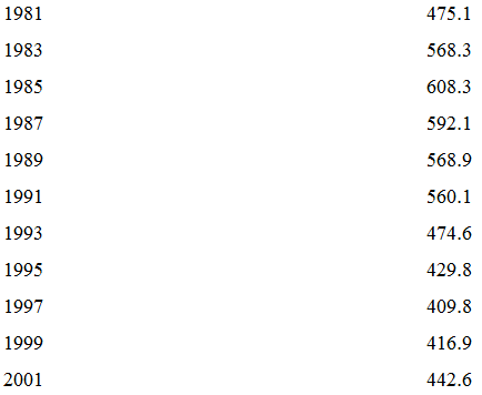
| 1981 | 475.1 |
| 1983 | 568.3 |
| 1985 | 608.3 |
| 1987 | 592.1 |
| 1989 | 568.9 |
| 1991 | 560.1 |
| 1993 | 474.6 |
| 1995 | 429.8 |
| 1997 | 409.8 |
| 1999 | 416.9 |
| 2001 | 442.6 |
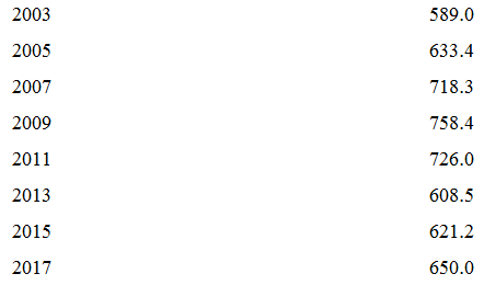
| 2003 | 589.0 |
| 2005 | 633.4 |
| 2007 | 718.3 |
| 2009 | 758.4 |
| 2011 | 726.0 |
| 2013 | 608.5 |
| 2015 | 621.2 |
| 2017 | 650.0 |
Graph:
A time-series plot for the given data is given by
b.
To find:The decade during which the national defence spending increasing and the decade during which the national defence spending increasing.
Answer to Problem 27E
The trend in the vacancy rate during the time period from 2012 to 2015 is decreasing.
Explanation of Solution
Solution:
A time-series plot for the given data is given by
From the time-series plot, we can see that during 1960s, 1980s and 2000s, the national defence spending is increasing and during 1950s, 1970s, 1990s and 2010s, the national defence spending is decreasing
Hence,
Increased decade: 1960s, 1980s and 2000s
Decreased decade: 1950s, 1970s, 1990s and 2010s.
c.
To find: The effects of the end of the war have on military spending after 1953.
Answer to Problem 27E
The effects of the end of the war have on military spending after 1953 is that it caught a big decrease.
Explanation of Solution
Solution:
A time-series plot for the given data is given by
From the time-series plot, we can see that after 1953, there was causing a big decrease in the military spending. The military spending was falling from 531.9 to 411.9 during 1953-1955.
Hence, the effects of the end of the war have on military spending after 1953 is that there caused a big decrease.
d.
To explain: The reflection in the national defence spending from 1965 to 1975.
Answer to Problem 27E
The national defence spending is increased from 1965 to 1969 and then decreased from 1969 to 1975.
Explanation of Solution
Given information: The following table presents the amount spent, in billions of dollars, on national defence by the U.S. government every other year for the years 1951 through 2017. The amounts are adjusted for inflation, and represent 2017 dollars.
| Year | Spending |
| 1951 | 503.1 |
| 1953 | 531.9 |
| 1955 | 411.9 |
| 1957 | 438.2 |
| 1959 | 432.4 |
| 1961 | 437.6 |
| 1963 | 470.9 |
| 1965 | 447.1 |
| 1967 | 569.3 |
| 1969 | 572.6 |
| 1971 | 476.8 |
| 1973 | 436.9 |
| 1975 | 404.0 |
| 1977 | 427.9 |
| 1979 | 424.4 |
| 1981 | 475.1 |
| 1983 | 568.3 |
| 1985 | 608.3 |
| 1987 | 592.1 |
| 1989 | 568.9 |
| 1991 | 560.1 |
| 1993 | 474.6 |
| 1995 | 429.8 |
| 1997 | 409.8 |
| 1999 | 416.9 |
| 2001 | 442.6 |
| 2003 | 589.0 |
| 2005 | 633.4 |
| 2007 | 718.3 |
| 2009 | 758.4 |
| 2011 | 726.0 |
| 2013 | 608.5 |
| 2015 | 621.2 |
| 2017 | 650.0 |
During the period 1965-1968, the United States steadily increased the number of troops in Vietnam from 23,000 at the beginning of 1965 to 537,000 at the end of 1968. Beginning in 1969, the number of Americans in Vietnam was steadily reduced, with the last of themleaving in 1975.
A time-series plot for the given data is given by
From 1965 to 1975, the national defence spending is increasing from 1965 to 1969 and then decreasing from 1969 to 1975.
Hence, the national defence spending is increased from 1965 to 1969 and then decreased from 1969 to 1975.
Want to see more full solutions like this?
Chapter 2 Solutions
Elementary Statistics ( 3rd International Edition ) Isbn:9781260092561


- Table 6 shows the year and the number ofpeople unemployed in a particular city for several years. Determine whether the trend appears linear. If so, and assuming the trend continues, in what year will the number of unemployed reach 5 people?arrow_forwardThe Hungry Person restaurant has posted its sales (in thousands of dollars) for the last two years. Month 1st Year 2nd Year January 201 216 February 216 223 March 232 240 April 201 244 May 221 232 June 213 220 July 220 211 August 214 213 September 202 217 October 217 220 November 224 212 December 236 216 a) Construct a time series plot in excel. (Label axes and graph) b) Develop a four month moving average. Compute MSE and forecast the amount of sales for the next month. c) Use α = 0.2 to compute the exponential smoothing values. Compute MSE and forecast for the next month. d) Compare the result for the four month average and exponential smoothing. Which appears to provide a better forecast based on MSE? Explain.arrow_forwardA statistical program is recommended. The quarterly sales data (number of copies sold) for a college textbook over the past three years follow. Quarter Year 1 Year 2 Year 3 1 1,690 1,800 1,860 2 950 910 1,110 3 2,625 2,910 2,940 4 2,510 2,370 2,615 (a) Construct a time series plot. What type of pattern exists in the data? There appears be a downward linear trend but no seasonal pattern in the data.There appears to be a seasonal pattern in the data and perhaps a moderate upward linear trend. There appears be an upward linear trend but no seasonal pattern in the data.There appears to be a seasonal pattern in the data and perhaps a moderate downward linear trend. (b) Use a regression model with dummy variables as follows to develop an equation to account for seasonal effects in the data. (Round your numerical values to the nearest integer.) Qrt1 = 1 if quarter 1, 0 otherwise; Qrt2 = 1 if quarter 2, 0 otherwise; Qrt3 = 1 if quarter 3, 0 otherwise t =…arrow_forward
- The Vintage Restaurant, on Captive Island near Fort Meyers, Florida, is owned and operated by Karen Payne. The restaurant just completed its second year of operation. Below are the sales for those two years (in ten thousands of dollars). Month First Year Second Year January 57 61 February 51 75 March 58 54 April 57 56 May 68 62 June 72 71 July 60 59 August 51 75 September 68 68 October 51 50 November 71 64 December 75 58 a) Construct a time-series plot in excel. (Label axes and graph) b) Develop a six month moving average. Compute MSE and forecast the amount of sales for the next month. c) Use α = 0.2 to compute the exponential smoothing values. Compute MSE and forecast for the next month. d) Compare the result for the six month average and exponential smoothing. Which appears to provide a better…arrow_forwardConsider the following time series. Quarter Year 1 Year 2 Year 3 1 70 67 61 2 50 42 52 3 59 61 54 4 79 82 73 (a) Construct a time series plot. What type of pattern exists in the data? Is there an indication of a seasonal pattern? The time series plot shows a horizontal pattern, but there is also a seasonal pattern in the data.The time series plot shows a horizontal pattern with no seasonal pattern present. The time series plot shows a trend pattern, but there is also a seasonal pattern in the data.The time series plot shows a trend pattern with no seasonal pattern present. (b) Use a multiple linear regression model with dummy variables as follows to develop an equation to account for seasonal effects in the data. x1 = 1 if quarter 1, 0 otherwise; x2 = 1 if quarter 2, 0 otherwise; x3 = 1 if quarter 3, 0 otherwise. ŷ = (c) Compute the quarterly forecasts for the next year. quarter 1 forecast quarter 2 forecast quarter 3 forecast quarter 4 forecastarrow_forwardWhich of the following time periods will have the largest annual average increase in the percentage of jobs that could be fully automated (based on the provided images attached)? A) 2020-2028 B) 2028-2030 C) 2030-2035 D) 2035-2040 E) 2040-2050 Transcribed Image Text:Preparing for Automation The possibility of having robots or mechanical assistants completing our laborious, dangerous, or repetitive day-to-day tasks has long been a dream of humanity. Now, as Robotic Process Automation (RPA) becomes commonplace, this dream or concern, depending on viewpoint - is getting closer. RPA, far from the walking, talking android commonly found in science fiction series, can be thought of as a programmable piece of software which, through using a series of rules, will complete repetitive tasks with a lower error rate and less interruption than a human completing the same tasks. The aim of RPA, beyond improving efficiency, is to free up humans from the monotony of roles like data entry, stock…arrow_forward
- The number of users of a certain website (in millions) from 2004 through 2011 follows. Year Period Users (Millions) 2004 1 1 2005 2 5 2006 3 11 2007 4 59 2008 5 146 2009 6 360 2010 7 608 2011 8 846 (a) Construct a time series plot. -A time series plot contains a series of 8 points connected by line segments. The horizontal axis ranges from 0 to 10 and is labeled: Period. The vertical axis ranges from 0 to 900 and is labeled: Millions of Users. The first point is at approximately (1, 850). The rest are plotted from left to right at regular increments of 1 period in a downward, diagonal direction that becomes less steep as period increases. The last point is at approximately (8, 0). -A time series plot contains a series of 8 points connected by line segments. The horizontal axis ranges from 0 to 10 and is labeled: Period. The vertical axis ranges from 0 to 900 and is labeled: Millions of Users. The first point is at approximately (1, 0). The rest are…arrow_forwardcorporate triple-a bond interest rates for 12 consecutive months follow.9.5 9.3 9.4 9.6 9.8 9.7 9.8 10.5 9.9 9.7 9.6 9.6a. construct a time series plot. What type of pattern exists in the data?arrow_forwardAfter its move in 1990 to La Junta, Colorado, and its new initiatives, the DeBourgh Manufacturing Company began an upward climb of record sales. Suppose the figures shown here are the DeBourgh monthly sales figures from January 2001 through December 2009 (in $1,000s). a) Produce a time series plot. Are there any trends evident in the data? Does DeBourgh have a seasonal component to its sales? b) Deseasonalize the data using Multiplicative model with a 0.5 weighted moving average. Produce a time series plot of the deseasonalized data and add a trendline. c) Forecast the sales from January to December of the year 2010. d) Include a discussion of the general direction of sales and any seasonal tendencies that might be occurrinG Month 2001 2002 2003 2004 2005 2006 2007 2008 2009 January 139.7 165.1 177.8 228.6 266.7 431.8 381 431.8 495.3 February 114.3 177.8 203.2 254 317.5 457.2 406.4 444.5 533.4 March 101.6 177.8 228.6 266.7 368.3 457.2 431.8 495.3 635 April 152.4 203.2…arrow_forward
- The Energy Information Administration of the U.S. Department of Energy providedtime series data for the U.S. average price per gallon of conventional regular gasolinebetween January 2007 and February 2014 (Energy Information Administration website,March 2014). Use the Internet to obtain the average price per gallon of conventionalregular gasoline since February 2014.a. Extend the graph of the time series shown in Figure 1.1.b. What interpretations can you make about the average price per gallon of conventionalregular gasoline since February 2014?c. Does the time series continue to show a summer increase in the average price pergallon? Explain.arrow_forward40. In the theory of time series, earthquakes can be considered as a. Secular Trend b. Cyclical Variation c. Seasonal Variation d. Irregular Variationsarrow_forwardUnited Dairies, Inc., supplies milk to several independent grocers throughout DadeC ounty, Florida. Managers at United Dairies want to develop a forecast of the number ofhalf gallons of milk sold per week. Sales data for the past 12 weeks are: a. Construct a time series plot. What type of pattern exists in the data?b. Use exponential smoothing with a 5 0.4 to develop a forecast of demand for week 13.What is the resulting MSE?arrow_forward
 Elementary AlgebraAlgebraISBN:9780998625713Author:Lynn Marecek, MaryAnne Anthony-SmithPublisher:OpenStax - Rice University
 College Algebra (MindTap Course List)AlgebraISBN:9781305652231Author:R. David Gustafson, Jeff HughesPublisher:Cengage Learning