NUMERICAL METH. F/ENGR.(LL)--W/ACCESS
7th Edition
ISBN: 9781260514131
Author: Chapra
Publisher: MCG
bartleby

Concept explainers

bartleby

Videos

Textbook Question
Book Icon
Chapter 25, Problem 1P

Solve the following initial value problem over the interval from t = 0  to 2 where  y ( 0 ) = 1 . Display all your results on the same graph.

d y d t = y t 2 1.1 y

(a) Analytically.

(b) Euler's method with h = 0.5  and 0 .25 .

(c) Midpoint method with h = 0.5 .

(d) Fourth-order RK method with h = 0.5 .

(a)

Expert Solution
Check Mark
To determine

To calculate: The solution of the initial value problem dydt=yt21.1y with the initial condition as y(0)=1, analytically.

Answer to Problem 1P

Solution:

The solution to the initial value problem is y(t)=et331.1t+C.

Explanation of Solution

Given Information:

The initial value problem dydt=yt21.1y where y(0)=1.

Formula used:

Tosolve an initial value problem of the form dydx=g(x)h(y) integrate both sides of the following equation:

dyh(y)=g(x)dx

Calculation:

Rewrite the provided differential equation as,

dydt=yt21.1ydydt=y(t21.1)dyy=(t21.1)dt

Integrate both sides to get,

lny=t331.1t+Cy(t)=et331.1t+C

Now use the initial condition y(0)=1 to get the value of constant C.

y(0)=e0331.1(0)+C1=1+CC=0

Hence, the analytical solution of the initial value problem is y(t)=et331.1t.

(b)

Expert Solution
Check Mark
To determine

To calculate: The solution of the initial value problem dydt=yt21.1y with the initial condition as y(0)=1 in the interval t(0,2) with step-sizes 0.5 and 0.25 using the Euler’s method.

Answer to Problem 1P

Solution:

For h=0.5 the values are,

t y dydt
0 1 1.1
0.5 0.45 0.3825
1 0.25875 0.02588
1.5 0.245813 0.282684
2 0.387155 1.122749

And, for h=0.25 the values are,

t y dydt
0 1 1.1
0.25 0.725 0.75219
0.5 0.536593 0.45641
0.75 0.422861 0.22728
1 0.36603 0.0366
1.25 0.356879 0.165057
1.5 0.398143 0.457865
1.75 0.51261 1.005997
2 0.764109 2.215916

Explanation of Solution

Given Information:

The initial value problem dydt=yt21.1y, with y(0)=1 in the interval t(0,2) with step-size 0.5.

Formula used:

Solve an initial value problem of the form dydx=f(xi,yi) using the iterative Euler method as,

yi+1=yi+f(xi,yi)h

Calculation:

From the initial condition y(0)=1, y0=1,t0=0, thus,

f(1,0)=(1)(0)21.1(1)=1.1

Let h=0.5, thus,

y1=y0+f(y0,t0)hy(0.5)=y(0)+f(1,0)0.5=11.1(0.5)=0.45

Proceed further and use the following MATLAB code to implement Euler’s method and solve the differential equation.

% Q 1 (b) Euler's Method when h=0.5 and 0.25

clear;clc;

% Define the end-points of the interval [0,2]

a=0;b=2;

% Define the initial condition y(0)=1

y1(1)=1;y2(1)=1;

t1(1)=a;t2(1)=a;

dydt(1)=-1.1;

% Mention the step-size as 0.5 or 0.25

h1=0.5;h2=0.25

% Compute the value of the number of iterations corresponding to the step-size;

n1=(b-a)/h1;

n2=(b-a)/h2;

% Start the loop for the Euler's method

fori=1:n1

% Compute the value of the function to the right of

% the differential equation

dydt1(i+1)=(y1(i)*t1(i)*t1(i)-1.1*y1(i));

% Compute the value of the variable y

y1(i+1)=y1(i)+h1*dydt1(i+1);

% Compute the value of the variable t

t1(i+1)=t1(i)+h1;

end

% Display the results:

A1=[t1;y1;dydt1]'

fori=1:n2

% Compute the value of the function to the right of the % differentialequation

dydt2(i+1)=(y2(i)*t2(i)*t2(i)-1.1*y2(i));

% Compute the value of the variable y

y2(i+1)=y2(i)+h2*dydt2(i+1);

% Compute the value of the variable t

t2(i+1)=t2(i)+h2;

end

A2=[t2;y2;dydt2]'

t1=linspace(0,2);

exactsol=exp(((t1.^3)/3)-1.1*t1);

plot(t1, exactsol)

axis([0 2 0 2])

hold on

plot(A1(:,1), A1(:,2));hold on

plot(A2(:,1), A2(:,2))

xlabel('t')

legend('y(t)','h=0.5','h=0.25')

Execute the above code to obtain the solutions for h=0.5 tabulated as,

t y dydt
0 1 1.1
0.5 0.45 0.3825
1 0.25875 0.02588
1.5 0.245813 0.282684
2 0.387155 1.122749

Now, the similar procedure can be followedfor the step size h=0.25.

The results thus obtained are tabulated as,

t y dydt
0 1 1.1
0.25 0.725 0.75219
0.5 0.536593 0.45641
0.75 0.422861 0.22728
1 0.36603 0.0366
1.25 0.356879 0.165057
1.5 0.398143 0.457865
1.75 0.51261 1.005997
2 0.764109 2.215916

The results for the two-step-sizes are plotted along with the analytical solution y(t)=et331.1t+C as shown below,

NUMERICAL METH. F/ENGR.(LL)--W/ACCESS, Chapter 25, Problem 1P , additional homework tip  1

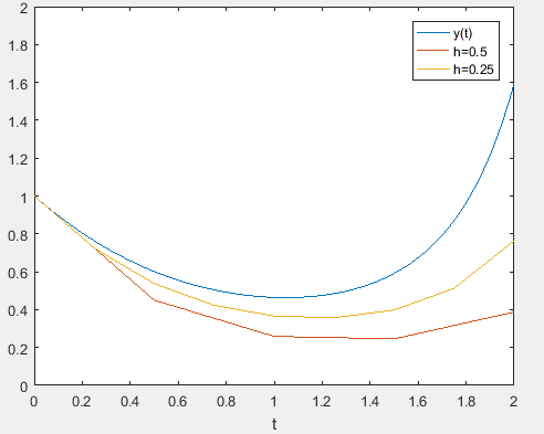
It is inferred that the smaller step-size would give a better approximation to the solution.

(c)

Expert Solution
Check Mark
To determine

To calculate: The solution of the initial value problem dydt=yt21.1y with initial condition as y(0)=1 in the interval t(0,2) and with the step-size of 0.5 using the mid-point method.

Answer to Problem 1P

Solution:

The solutions are tabulated as,

t y dydt
0 1 1.1
0.5 0.623906 0.53032
1 0.491862 0.04919
1.5 0.602762 0.693176
2 1.364267 3.956374

Explanation of Solution

Given Information:

The initial value problem dydt=yt21.1y, with y(0)=1 in the interval t(0,2) and with the step-size of 0.5.

Formula used:

Solve an initial value problem of the form dydx=f(xi,yi) using the iterative mid-point method as,

yi+1=yi+f(xi+0.5,yi+0.5)h

Here,

yi+0.5=yi+f(xi,yi)h2

Calculation:

From the initial condition y(0)=1, y0=1,t0=0.

f(y0,t0)=f(1,0)=(1)(0)21.1(1)=1.1

Let h=0.5. Thus,

y0+0.5=y0+f(x0,y0)h2=11.1(0.5)2=0.725

Now,

f(y0.5,t0.5)=f(0.725,0.25)=(0.725)(0.25)21.1(0.725)=0.75219

Proceed further and use the following MATLAB code to implement mid-point iterative scheme and solve the differential equation.

% Q 1 (c) Midpoint Method when h=0.5

clear;clc;

% Define the end-points of the interval [0,2]

a=0;b=2;

% Define the initial condition y(0)=1

y1(1)=1;

t1(1)=a;

% Mention the step-size as 0.5

h1=0.5;

% Compute the value of the number of iterations corresponding to the step-size;

n1=(b-a)/h1;

% Start the loop for the Euler's method

fori = 1: n1

% the value of the right hand side of the DE

b(i)=f1(t1(i), y1(i,:));

% Increment in t

t1(i+1) = t1(i) + h1;

% The formula for the Midpoint method

z = y1(i,:) + (h1/2) * b(i);

y1(i+1,:) = y1(i,:) + h1 * f1(t1(i)+(h1/2), z);

end

% Display the results:

A=[t1' y1]

t1=linspace(0,2);

exactsol=exp(((t1.^3)/3)-1.1*t1);

plot(t1, exactsol)

axis([0 2 0 2])

hold on

plot(A(:,1), A(:,2));

legend('y(t)','mid-point')

Execute the above code to obtain the solutions tabulated as,

t Y dydt
0 1 1.1
0.5 0.623906 0.53032
1 0.491862 0.04919
1.5 0.602762 0.693176
2 1.364267 3.956374

The results for the are plotted along with the analytical solution y(t)=et331.1t+C as shown below,

NUMERICAL METH. F/ENGR.(LL)--W/ACCESS, Chapter 25, Problem 1P , additional homework tip  2

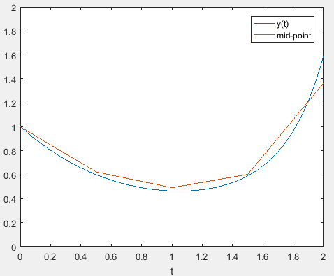
Thus, it is inferred that the mid-point method gives a good approximation to the solution.

(d)

Expert Solution
Check Mark
To determine

To calculate: The solution of the initial value problem dydt=yt21.1y with the initial condition as y(0)=1 in the interval t(0,2) with step-size of 0.5 using the fourth order RK method.

Answer to Problem 1P

Solution:

The solutions are tabulated as,

t y k1 k2 k3 k4
0 1 1.1 0.7522 0.8424 0.4920
0.5 0.6016 0.5113 0.2546 0.2891 0.0457
1 0.4645 0.0465 0.2095 0.2391 0.6717
1.5 0.5914 0.6801 1.4953 1.8937 4.4609
2 1.5845 4.5949 10.8302 17.0071 51.9532

Explanation of Solution

Given Information:

The initial value problem dydt=yt21.1y, with y(0)=1 in the interval t(0,2) and with the step-sizes of 0.5 and 0.25.

Formula used:

Solve an initial value problem of the form dydx=f(xi,yi) using the iterative fourth order RK method as,

yi+1=yi+16(k1+2k2+2k3+k4)h

In the above expression,

k1=f(xi,yi)k2=f(xi+h2,yi+h2k1)k3=f(xi+h2,yi+h2k2)k4=f(xi+h,yi+k3h)

Calculation:

From the initial condition y(0)=1, y0=1,t0=0.

k1=f(y0,t0)=f(1,0)=(1)(0)21.1(1)=1.1

Let h=0.5. Thus,

k2=f(t0+0.52,y0+(0.52)k1)=f(0.25,0.725)=0.7522

And,

k3=f(t0+0.52,y0+(0.52)k2)=f(0.25,0.812)=0.8424

And,

k4=f(t0+0.5,y0+0.5k3)=f(0.5,0.5788)=0.492

Therefore,

y1=y0+16(k1+2k2+2k3+k4)(0.5)=1+16(1.1+2(0.7522)+2(0.8424)+(0.492))(0.5)=0.6016

Proceed further and use the following MATLAB code to implement RK method of order four, solve the differential equation.

% Q 1 (d) RK 4 Method when h=0.5

clear;clc;

% Define the end-points of the interval [0,2]

a=0;b=2;

% Define the initial condition y(0)=1

y1(1)=1;

t1(1)=a;

% Mention the step-size as 0.5

h1=0.5;

% Compute the value of the number of iterations corresponding to the step-size;

n1=(b-a)/h1;

halfh = h1 / 2;

h6 = h1/6;

% Start the process

fori = 1: n1+1

t1(i+1) = t1(i) + h1;

th2 = t1(i) + halfh;

% The values usually defined as k1, k2, k3 and k4

s1(i) = f1(t1(i), y1(i,:));

s2(i) = f1(th2, y1(i,:) + halfh * s1(i));

s3(i) = f1(th2, y1(i,:) + halfh * s2(i));

s4(i) = f1(t1(i+1), y1(i,:) + h1 * s3(i));

% The formula for the RK method of order 4

y1(i+1,:) = y1(i,:) + (s1(i) + s2(i)+s2(i) + s3(i)+s3(i) + s4(i)) * h6;

end;

t1(:, end:end)=[];

y1(end:end,:)=[];

% Display the values

A=[t1' y1 s1' s2' s3' s4']

% Plot the graph of the exact solution along with the approximations

t1=linspace(0,2);

exactsol=exp(((t1.^3)/3)-1.1*t1);

plot(t1, exactsol)

axis([0 2 0 2])

hold on

plot(A(:,1), A(:,2));

xlabel('t')

legend('y(t)','RK4')

In an another .m file, define the equation as,

functionfunc=f1(t, y)

func=y*t^2-1.1*y;

Execute the above code to obtain the solutions tabulated as,

t y k1 k2 k3 k4
0 1 1.1 0.7522 0.8424 0.4920
0.5 0.6016 0.5113 0.2546 0.2891 0.0457
1 0.4645 0.0465 0.2095 0.2391 0.6717
1.5 0.5914 0.6801 1.4953 1.8937 4.4609
2 1.5845 4.5949 10.8302 17.0071 51.9532

The results for the are plotted along with the analytical solution y(t)=et331.1t+C.

NUMERICAL METH. F/ENGR.(LL)--W/ACCESS, Chapter 25, Problem 1P , additional homework tip  3

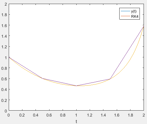
Hence, it is inferred that the RK method of order four gives the best approximation to the solution.

Want to see more full solutions like this?

Subscribe now to access step-by-step solutions to millions of textbook problems written by subject matter experts!

Chapter 25 Solutions

NUMERICAL METH. F/ENGR.(LL)--W/ACCESS

Knowledge Booster
Background pattern image
Advanced Math
Learn more about
Need a deep-dive on the concept behind this application? Look no further. Learn more about this topic, advanced-math and related others by exploring similar questions and additional content below.
Recommended textbooks for you
Text book image
Advanced Engineering Mathematics
Advanced Math
ISBN:9780470458365
Author:Erwin Kreyszig
Publisher:Wiley, John & Sons, Incorporated
Text book image
Numerical Methods for Engineers
Advanced Math
ISBN:9780073397924
Author:Steven C. Chapra Dr., Raymond P. Canale
Publisher:McGraw-Hill Education
Text book image
Introductory Mathematics for Engineering Applicat...
Advanced Math
ISBN:9781118141809
Author:Nathan Klingbeil
Publisher:WILEY
Text book image
Mathematics For Machine Technology
Advanced Math
ISBN:9781337798310
Author:Peterson, John.
Publisher:Cengage Learning,
Text book image
Basic Technical Mathematics
Advanced Math
ISBN:9780134437705
Author:Washington
Publisher:PEARSON
Text book image
Topology
Advanced Math
ISBN:9780134689517
Author:Munkres, James R.
Publisher:Pearson,
01 - What Is A Differential Equation in Calculus? Learn to Solve Ordinary Differential Equations.; Author: Math and Science;https://www.youtube.com/watch?v=K80YEHQpx9g;License: Standard YouTube License, CC-BY
Higher Order Differential Equation with constant coefficient (GATE) (Part 1) l GATE 2018; Author: GATE Lectures by Dishank;https://www.youtube.com/watch?v=ODxP7BbqAjA;License: Standard YouTube License, CC-BY
Solution of Differential Equations and Initial Value Problems; Author: Jefril Amboy;https://www.youtube.com/watch?v=Q68sk7XS-dc;License: Standard YouTube License, CC-BY