
Videos
Perform the same computation for the Lorenz equations in Sec. 28.2, but use (a) Euler's method, (b) Heun's method (without iterating the corrector), (c) the fourth-order RK method, and (d) the MATLAB ode45 function. In all cases use single-precision variables and a step size of 0.1 and simulate from
(a)
To calculate: The solution of Lorentz equation
Answer to Problem 18P
Solution:
The solution of Lorentz equations by the Euler’s method with step size 0.1 gives unstable solution.
Explanation of Solution
Given Information:
Lorentz equations,
and Initial conditions are
Formula used:
Euler’s method for
Where, h is the step size.
Calculation:
Consider the equations,
The iteration formula for Euler’s method with step size
Use excel to find all the iteration with step size
Step 1: Name the column A as t and go to column A2 and put 0 then go to column A3 and write the formula as,
=A2+0.1
Then, Press enter and drag the column up to
Step 2: Now name the column B as x-Euler and go to column B2 and write 5 and then go to the column B3 and write the formula as,
=B2+0.1*(-10*B2+10*C2)
Step 3: Press enter and drag the column up to
Step 4: Now name the column C as y-Euler and go to column C2 and write 5 and then go to the column C3 and write the formula as,
=C2+0.1*(28*B2-C2-B2*D2)
Step 5: Press enter and drag the column up to
Step 6: Now name the column D as z-Euler and go to column D2 and write 5 and then go to the column D3 and write the formula as,
=D2+0.1*(-2.666667*D2+B2*C2)
Step 7: Press enter and drag the column up to
Thus, first few iterations are as shown below,
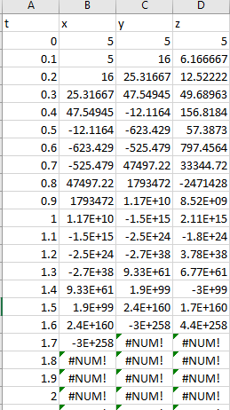
From the above result, it is observed that the solution of Lorentz equations by the Euler’s method with step size 0.1 the values are continuously decreasing. Hence, Euler method with step size 0.1 gives unstable solution for the Lorentz equations.
(b)
To calculate: The solution of Lorentz equation
Answer to Problem 18P
Solution:
The solution of Lorentz equations by the Heun’s method with step size 0.1 gives unstable solution.
Explanation of Solution
Given Information:
Lorentz equations,
and Initial conditions are
Formula used:
The iteration formula for Heun’s method is,
Calculation:
Consider the equations,
The following VBA code is used to solve the Lorentz equation by Heun’s method:
Code:
Output:
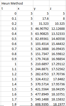
To draw the graph of the above results, follow the steps in excel sheet as given below,
Step 1: Select the cell from A4 to A205 and cell B4 to B205. Then, go to the Insert and select the scatter with smooth lines from the chart.
Step 2: Select the cell from A4 to A205 and cell C4 to C205. Then, go to the Insert and select the scatter with smooth lines from the chart.
Step 2: Select the cell from A4 to A205 and cell D4 to D205. Then, go to the Insert and select the scatter with smooth lines from the chart.
Step 4: Select one of the graphs and paste it on another graph to merge the graphs.
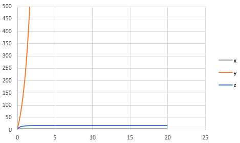
The graph obtained is,
And, to draw the phase plane plot follow the steps as below,
Step 4: Select the column B, column C and column D. Then, go to the Insert and select the scatter with smooth lines from the chart.
The graph obtained is,
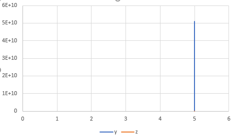
The phase plane plot is a straight line because solution of x is a constant value. The solution o0f Lorentz equation by Heun’s method with step size 0.1 is thus unstable.
(c)
To calculate: The solution of Lorentz equation
Answer to Problem 18P
Solution:
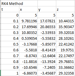
The first few solutions of Lorentz equation are,
| t | x | y | z |
| 0 | 5 | 5 | 5 |
| 0.1 | 9.781196 | 17.07821 | 10.44315 |
| 0.2 | 17.69946 | 20.86553 | 35.90347 |
| 0.3 | 10.80352 | -2.53933 | 39.32018 |
| 0.4 | 0.539054 | -5.55832 | 28.10261 |
| 0.5 | -3.17668 | -5.85077 | 22.41242 |
| 0.6 | -5.5818 | -8.41419 | 19.9751 |
| 0.7 | -8.8743 | -12.6404 | 22.17497 |
| 0.8 | -11.8816 | -13.3924 | 29.76851 |
| 0.9 | -10.6546 | -7.2405 | 33.36662 |
| 1 | -6.86073 | -3.45687 | 29.32358 |
Explanation of Solution
Given Information:
Lorentz equations,
and Initial conditions are
Formula used:
The fourth-order RK method for
Where,
Calculation:
The following VBA code is used to find the solution of Lorentz equation by the fourth order RK method:
Code:
Output:
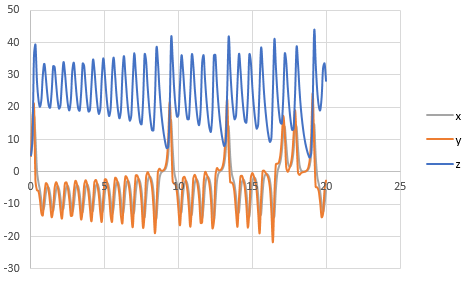
To draw the graph of the above results, follow the steps in excel sheet as given below,
Step 1: Select the cell from A4 to A205 and cell B4 to B205. Then, go to the Insert and select the scatter with smooth lines from the chart.
Step 2: Select the cell from A4 to A205 and cell C4 to C205. Then, go to the Insert and select the scatter with smooth lines from the chart.
Step 3: Select the cell from A4 to A205 and cell D4 to D205. Then, go to the Insert and select the scatter with smooth lines from the chart.
Step 4: Select one of the graphs and paste it on another graph to merge the graphs.
The graph obtained is,
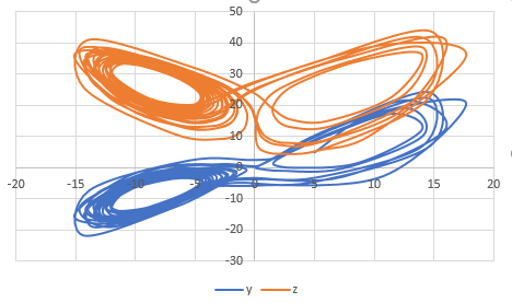
And, to draw the phase plane plot follow the steps as below,
Step 4: Select the column B, column C and column D. Then, go to the Insert and select the scatter with smooth lines from the chart.
The graph obtained is,
(d)
The solution of Lorentz equation
Answer to Problem 18P
Solution:
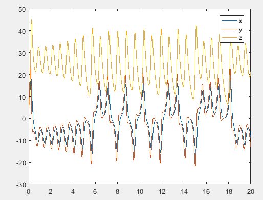
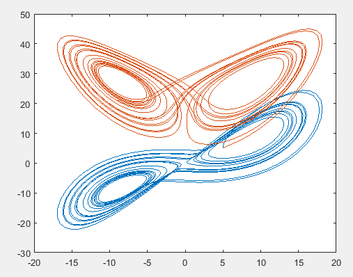
The solution graph of Lorentz equation is,
Explanation of Solution
Given Information:
Lorentz equations,
and Initial conditions are
Consider the Lorentz equations,
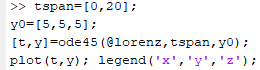
Use MATLAB ode45 function to solve the above differential functions as below,
Code:
Output:
The graph obtained as,
Write the command as below to plot the phase-plane,

The phase plane graph obtained as,
Want to see more full solutions like this?
Chapter 28 Solutions
Numerical Methods for Engineers
Additional Math Textbook Solutions
Advanced Engineering Mathematics
Basic Technical Mathematics
Fundamentals of Differential Equations (9th Edition)
Excursions in Modern Mathematics (9th Edition)
Precalculus: Mathematics for Calculus (Standalone Book)


 Advanced Engineering MathematicsAdvanced MathISBN:9780470458365Author:Erwin KreyszigPublisher:Wiley, John & Sons, Incorporated
 Numerical Methods for EngineersAdvanced MathISBN:9780073397924Author:Steven C. Chapra Dr., Raymond P. CanalePublisher:McGraw-Hill Education
 Introductory Mathematics for Engineering Applicat...Advanced MathISBN:9781118141809Author:Nathan KlingbeilPublisher:WILEY
 Mathematics For Machine TechnologyAdvanced MathISBN:9781337798310Author:Peterson, John.Publisher:Cengage Learning,
