Chapter 3, Problem 11CRE

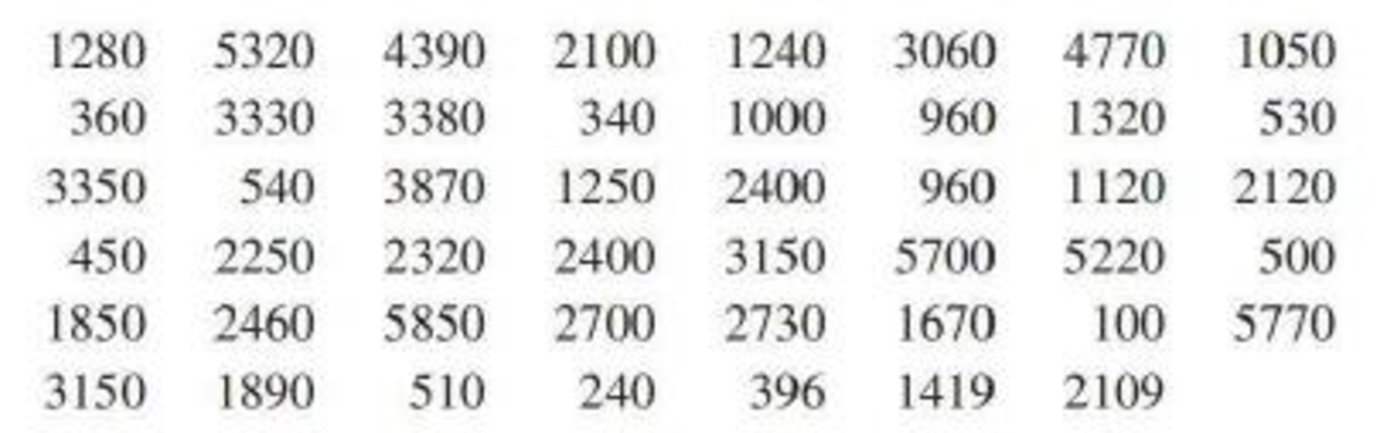
The article “Determination of Most Representative Subdivision” (Journal of Energy Engineering [1993]:44–55) gave data on various characteristics of subdivisions that could be used in deciding whether to provide electrical power using overhead lines or underground lines. Data on the variable x = total length of streets within a subdivision are as follows:

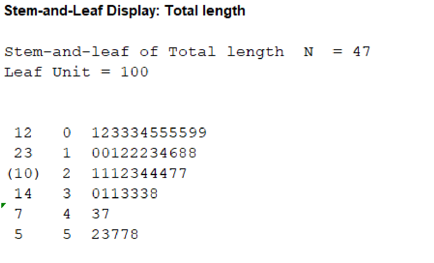
1. a. Construct a stem-and-leaf display for these data using the thousands digit as the stem. Comment on the various features of the display.
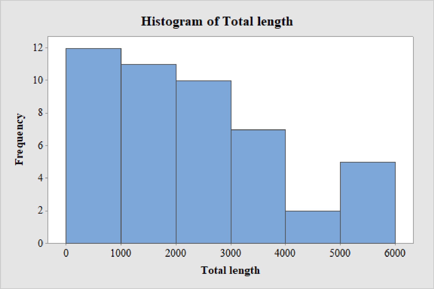
2. b. Construct a histogram using class boundaries of 0 to <1000, 1000 to <2000, and so on. How would you describe the shape of the histogram?
3. c. What proportion of subdivisions has total length less than 2000? between 2000 and 4000?

To determine

Draw the stem and leaf graph for the given data.

Comment on the interesting features of the graphical display.

Answer to Problem 11CRE

Output using MINITAB is given below:

Explanation of Solution

Calculation:

The data represents the total length of streets within a subdivision.

Here, it is given that the stems represent the thousands digit and leaves represent the hundreds digit.

Software procedure:

Step by step procedure to draw the stem and leaf graph using MINITAB software.

• Select Graph > Stem and leaf.
• Select Total length in Graph variables.
• Select OK.

Observation:

Here, the legend is $0|1=100$

Here, 0 represents stem and 1 represent leaf. That is, in the stem, 0 represent thousands place and 1 represents hundreds place. Thus, the required number is 100.

From the stem and leaf plot, it is observed that, the distribution of the data is positively skewed with single mode.

Representative value:

The representative value for the series of measurements is approximately the average of the remaining measurements excluding the outliers of the data set.

Here, from the stem and leaf plot it is observed that after removing the observations that are far away from each other. The average of the data points is approximately around 2,100.

Therefore, the representative gravity is 2,100.

Variation in the data set:

Generally the variation will be dependent on the range of the data set. Usually for large range the variation will be large.

The general formula for range is,

$\text{Range}=\text{maximum}\text{value}-\text{minimum value}$

From the stem and leaf plot it is observed that, the maximum and minimum values are 5,800 and 100.

The range of the strength of beams is,

$\begin{array}{c}\text{Range}=5,800-100\\ =5,700\end{array}$

Thus, the range is 5,700.

The representative value is 2,100, there is large variation between range and representative value.

Hence, the researchers conclude that the data contains reasonably large variation.

To determine

Draw the frequency histogram for the given data.

Describe the shape of the histogram.

Answer to Problem 11CRE

Output using MINITAB is given below.

Explanation of Solution

Calculation:

Here, the first lower bound should be 0 and the first upper bound should be 1,000.

The class width should be 10 and the number of classes should be 6.

That is, the class intervals are 0 – <1,000, 1,000 – <2,000, 2,000 – <3,000, 3,000 – <4,000, 4,000 – <5,000 and 5,000-<6,000.

Software procedure:

Step by step procedure to draw the histogram using MINITAB software.

• Select Graph > Histogram.
• Select Simple.
• Enter Total length in Graph variables.
• In edit X-scale, select Binning.
• Select Cut point in Interval type.
• Enter 6 in number of intervals.
• Enter the values of 0, 1,000, 2,000, 3,000, 4,000, 5,000 and 6,000 in midpoint/Cut point positions.
• Select OK.

Interesting features of the histogram:

From the histogram, it is observed that the distribution of total lengths is positively skewed with single mode.

• The distribution of total length is a unimodal distribution, since there is only one peak bar with the highest frequency on the histogram.
• The distribution of total length is positively skewed, that is, the length of the curve of the right-hand tail is higher than the left-hand tail.
• The minimum value of the total length is 100 and the maximum value of the percentages is 5,850.
• The range of the distribution of percentages is as follows:

  $\begin{array}{c}\text{Range = maximum }-\text{ minimum}\\ =5,850-100\\ =5,750\end{array}$.

• The variability is the distribution of total length is too high.
• The distribution of total length is centred around 2,100.

To determine

Find the proportion of subdivisions whose total length is less than 2,000.

Find the proportion of subdivisions whose total length is in between 2,000 and 4,000.

Answer to Problem 11CRE

The proportion of subdivisions whose total length is less than 2,000 is 0.4894.

The proportion of subdivisions whose total length is in between 2,000 and 4,000 is 0.3617.

Explanation of Solution

Calculation:

The general formula for the relative frequency or proportion is,

$\text{Relative}\text{Frequency or proportion = }\frac{\text{Frequency}}{\text{Total frequency}}$

Proportion of subdivisions whose total length is less than 2,000:

Here, the observations that correspond to the first two intervals are less than 2,000.

From the data, it is observed that the number of observations that are less than 2,000 is given below:

$\begin{array}{c}\text{Number}\text{of}\text{observations}\text{less}\text{than 2,000}=12+11\\ =23\end{array}$

The total number of observations is,

$\begin{array}{c}\text{Total}\text{number}\text{of}\text{observations}=12+11+10+7+2+5\\ =47\end{array}$

The proportion of subdivisions whose total length is less than 2,000 is obtained as given below:

Substituting the number of subdivisions whose total length is less than 2,000 is “23” as the frequency and total number of observations “47” as total frequency in relative frequency.

$\begin{array}{c}\left(\begin{array}{l}\text{Relative}\text{Frequency or proportion}\text{of}\text{subdivisions }\\ \text{whose total length is less than 2,000}\end{array}\right)=\frac{23}{47}\\ =0.4894\end{array}$

Thus, the proportion of subdivisions whose total length is less than 2,000 is 0.4894.

Proportion of subdivisions whose total length is in between 2,000 and 4,000:

Here, the observations that correspond to the third and fourth intervals are in between 2,000 and 4,000.

From the data, it is observed that the number of observations that are in between 2,000 and 4,000 is given below:

$\begin{array}{c}\text{Number}\text{of}\text{observations}\text{ between 2,000 and 4,000}=10+7\\ =17\end{array}$

The total number of observations is given below:

$\begin{array}{c}\text{Total}\text{number}\text{of}\text{observations}=12+11+10+7+2+5\\ =47\end{array}$

The proportion of subdivisions whose total length between 2,000 and 4,000 is obtained as given below:

Substituting the number of subdivisions whose total length between 2,000 and 4,000 is “17” as the frequency and total number of observations “47” as total frequency in relative frequency.

$\begin{array}{c}\left(\begin{array}{l}\text{Relative}\text{Frequency or proportion}\text{of}\text{subdivisions }\\ \text{whose total length is in between 2,000 and 4,000}\end{array}\right)=\frac{17}{47}\\ =0.3617\end{array}$

Thus, the proportion of subdivisions whose total length is in between 2,000 and 4,000 is 0.3617.