Numerical Methods for Engineers
7th Edition
ISBN: 9780073397924
Author: Steven C. Chapra Dr., Raymond P. Canale
Publisher: McGraw-Hill Education
bartleby

Concept explainers

bartleby

Videos

Textbook Question
Book Icon
Chapter 32, Problem 9P

The velocity of water flow through the porous media can be related to head by D'Arcy's law

q n = K d h d n

where K is the hydraulic conductivity and q n is discharge velocity in the n direction. If K = 5 × 10 4  cm/s , compute the water velocities for Prob. 32.8.

Expert Solution & Answer
Check Mark
To determine

To calculate: The water flowsvelocity through the porous media for the Prob. 32.8, if the hydraulic conductivity is K=5×104 cm/s.

Answer to Problem 9P

Solution:

The water flow velocity at every node is,

-5.205E-04 -5.542E-04 -6.593E-04 -7.249E-04
-5.079E-04 -5.315E-04 -6.989E-04 -7.942E-04
-4.668E-04 -3.967E-04 -4.429E-04

Explanation of Solution

Given Information:

Write the expression for D’Arcy’s law.

qn=Kdhdn

Here, K is the hydraulic conductivity and qn is the discharge velocity in n direction.

The hydraulic conductivity is K=5×104 cm/s.

Formula used:

Consider the Laplace Equation,

2hx2+2hy2=0

Write the central difference approximation for the second derivative.

hi+1,j2hi,j+hi1,jΔx2+hi,j+12hi,j+hi,j1Δy2=0

Calculation:

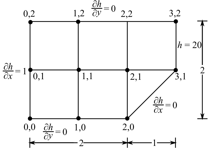
Refer to Figure P32.8, draw the nodal diagram.

Numerical Methods for Engineers, Chapter 32, Problem 9P

Recall the Laplace Equation,

2hx2+2hy2=0

The central difference approximation applies for the second derivative in above Laplace equation,

hi+1,j2hi,j+hi1,jΔx2+hi,j+12hi,j+hi,j1Δy2=0 …… (1)

At the node, (i,j)=(0,0) the equation (1) reduces to

h1,02h0,0+h1,0Δx2+h0,12h0,0+h0,1Δy2=0 …... (2)

Approximate the all external nodes with a central finite difference,

dhdy=h0,1h0,12Δyh0,1h0,1=2Δydhdy=2Δy0=0

Thus, h0,1=h0,1 …… (3)

Now with a central finite difference, approximate the external nodes.

dhdx=h1,0h1,02Δx2Δxdhdx=h1,0h1,0h1,0=h1,02Δxdhdx=h1,02×1×1

Solve further,

h1,0=h1,02 …… (4)

Substitute (3) and (4) in (2).

h1,02h0,0+(h1,02)Δx2+h0,12h0,0+h0,1Δy2=02h1,02h0,02Δx2+2h0,12h0,0Δy2=04h0,02h1,02h0,1=2

Similarly, at the node, (i,j)=(0,1) the equation (1) can write,

h0,0+4h0,1h0,22h1,1=2

Similarly, at the node, (i,j)=(0,2) the equation (1) can write,

2h0,1+4h0,22h1,2=2

Similarly, at the node, (i,j)=(1,0) the equation (1) can write,

h0,0+4h1,0h2,02h1,1=0

Similarly, at the node, (i,j)=(1,1) the equation (1) can write,

h0,1h1,0h1,2+4h1,1h2,1=0

Similarly, at the node, (i,j)=(1,2) the equation (1) can write,

h0,22h1,1+4h1,2h2,2=0

Similarly, at the node, (i,j)=(2,0) the equation (1) can write,

2h1,0+4h2,02h2,1=0

Similarly, at the node, (i,j)=(2,1) the equation (1) can write,

h2,0h1,1+4h2,1h2,2=20

Similarly, at the node, (i,j)=(2,2) the equation (1) can write,

h1,22h2,1+4h2,2=20

Thus, the system of all linear equations is,

4h0,02h1,02h0,1=2h0,0+4h0,1h0,22h1,1=22h0,1+4h0,22h1,2=2

And,

h0,0+4h1,0h2,02h1,1=0h0,1h1,0h1,2+4h1,1h2,1=0h0,22h1,1+4h1,2h2,2=0

And,

2h1,0+4h2,02h2,1=0h2,0h1,1+4h2,1h2,2=20h1,22h2,1+4h2,2=20

Write all equation in matrix form.

[422000000104102000002400002140012000011004101000102014020040200000011410000000241][h00h10h01h02h20h11h21h22h12]=[22200002020]

Use the MATLAB to solve the above equations, write the following code in MATLAB.

A =zeros(9,9);

A(1,1)=4;

A(1,2)=-2;

A(1,3)=-2;

A(2,1)=-1;

A(2,3)=4;

A(2,4)=-1;

A(2,6)=-2;

A(3,3)=-2;

A(3,4)=4;

A(3,9)=-2;

A(4,1)=-1;

A(4,2)=4;

A(4,5)=-1;

A(4,6)=-2;

A(5,2)=-1;

A(5,3)=-1;

A(5,6)=4;

A(5,7)=-1;

A(5,9)=-1;

A(6,4)=-1;

A(6,6)=-2;

A(6,8)=-1;

A(6,9)=4;

A(7,2)=-2;

A(7,5)=4;

A(7,7)=-2;

A(8,5)=-1;

A(8,6)=-1;

A(8,7)=4;

A(8,8)=-1;

A(9,7)=-2;

A(9,8)=4;

A(9,9)=-1;

%

b =[-2;-2;-2;0;0;0;0;20;20];

Sol = A\b

The output is,

Sol =

16.2279

17.1589

16.2969

16.3372

17.7853

17.3113

18.4117

18.5502

17.3775

[h00h10h01h02h20h11h21h22h12]=[ 16.2279 17.158916.296916.337217.785317.311318.411718.550217.3775]

Thus, the distribution of head of the system is shown below.

16.3372 17.37748 18.55022 20
16.29691 17.31126 18.4117 20
16.22792 17.15894 17.78532

Now from the above table find the value of dhdx and dhdy.

dhdx=khi+1,jhi1,j2Δx

And

dhdy=khi,j+1hi,j12Δy

Calculate the value of dhdx for every node.

(dhdx)0,2=h1,2h0,2=17.3374816.3372=1.04029

And,

(dhdx)0,1=h2,1h0,1=17.3112616.29691=1.01435

Calculate all the value of dhdx the same way for every node. After calculating all the values of dhdx the following table will be obtained:

1.04029 1.10651 1.31126 1.44978
1.01435 1.05740 1.34437 1.58830
0.93102 0.77870 0.62638

Calculate the value of dhdy for every node.

(dhdy)0,2=h0,2h0,1=16.337216.29691=0.04029

Calculate all the value of dhdy for every node same way. After calculating all the values of dhdy obtained the following table:

0.04029 0.06623 0.13852 0.00000
0.05464 0.10927 0.38245 0.00000
0.06898 0.15232 0.62638

Now calculate the value of dhdn.

dhdnn=dhdxn2+dhdyn2

Substitute the values of dhdx and dhdy for every node then the value of dhdn to the corresponding nodes will be obtained.

For (dhdn)0,2,

(dhdn)0,2=(dhdx)0,22+(dhdy)0,22=(1.04029)2+(0.04029)2=1.04107

Calculate for every node the value of dhdn same way. After calculating all the values obtained the following table.

1.04107 1.10849 1.31855 1.44978
1.01582 1.06303 1.39771 1.58830
0.93357 0.79345 0.88583

Apply the D’Arcy law to find the discharge velocity in the n direction:

qn=Kdhdn

Here, K=5×104 cm/s is the hydraulic conductivity.

Now Calculate for the velocity (q0,2).

q0,2=K(dhdn)0,2=(5×104 cm/s)×1.04107=5.205×105 cm/s

Calculate the velocity for every node same way, and got the following table:

-5.205E-04 -5.542E-04 -6.593E-04 -7.249E-04
-5.079E-04 -5.315E-04 -6.989E-04 -7.942E-04
-4.668E-04 -3.967E-04 -4.429E-04

Want to see more full solutions like this?

Subscribe now to access step-by-step solutions to millions of textbook problems written by subject matter experts!
Knowledge Booster
Background pattern image
Advanced Math
Learn more about
Need a deep-dive on the concept behind this application? Look no further. Learn more about this topic, advanced-math and related others by exploring similar questions and additional content below.
Recommended textbooks for you
Text book image
Mathematics For Machine Technology
Advanced Math
ISBN:9781337798310
Author:Peterson, John.
Publisher:Cengage Learning,
Text book image
Algebra & Trigonometry with Analytic Geometry
Algebra
ISBN:9781133382119
Author:Swokowski
Publisher:Cengage
Text book image
Trigonometry (MindTap Course List)
Trigonometry
ISBN:9781337278461
Author:Ron Larson
Publisher:Cengage Learning
Text book image
College Algebra
Algebra
ISBN:9781337282291
Author:Ron Larson
Publisher:Cengage Learning
Mod-01 Lec-01 Discrete probability distributions (Part 1); Author: nptelhrd;https://www.youtube.com/watch?v=6x1pL9Yov1k;License: Standard YouTube License, CC-BY
Discrete Probability Distributions; Author: Learn Something;https://www.youtube.com/watch?v=m9U4UelWLFs;License: Standard YouTube License, CC-BY
Probability Distribution Functions (PMF, PDF, CDF); Author: zedstatistics;https://www.youtube.com/watch?v=YXLVjCKVP7U;License: Standard YouTube License, CC-BY
Discrete Distributions: Binomial, Poisson and Hypergeometric | Statistics for Data Science; Author: Dr. Bharatendra Rai;https://www.youtube.com/watch?v=lHhyy4JMigg;License: Standard Youtube License