
Videos
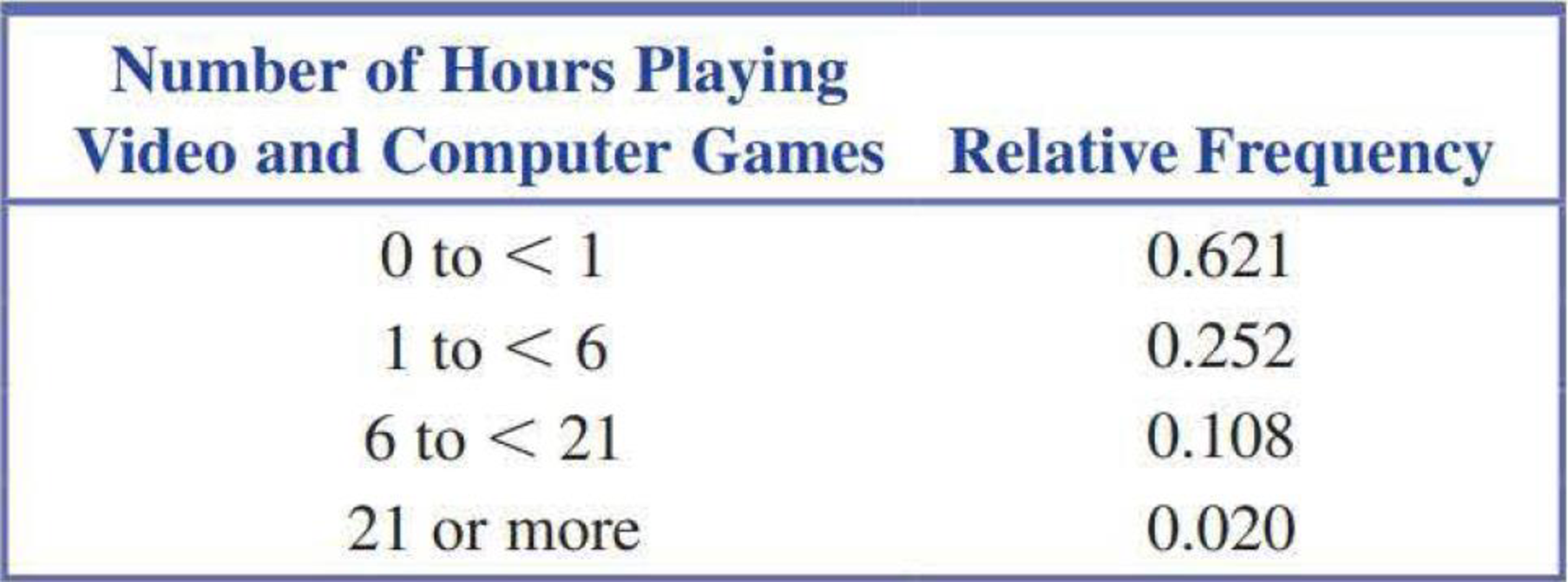
The following two relative frequency distributions are based on data that appeared in The Chronicle of Higher Education (August 23, 2013). The data are from a survey of students at four-year colleges. One relative frequency distribution is for the number of hours spent online at social network sites in a typical week. The second relative frequency distribution is for the number of hours spent playing video and computer games in a typical week.
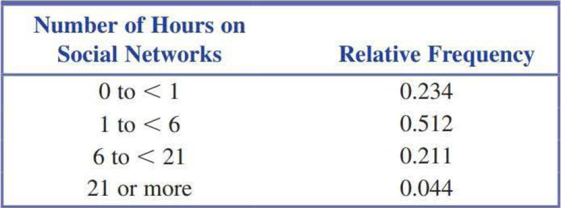
- a. Construct a histogram for the social media data. For purposes of constructing the histogram, assume that none of the students in the sample spent more than 40 hours on social media in a typical week and that the last interval can be regarded as 21 to <40. Be sure to use the density scale when constructing the histogram. (Hint: See Example 3.17.)
- b. Construct a histogram for the video and computer game data. Use the same scale that you used for the histogram in Part (a) so that it will be easy to compare the two histograms.
- c. Comment on the similarities and differences in the histograms from Parts (a) and (b).
a.
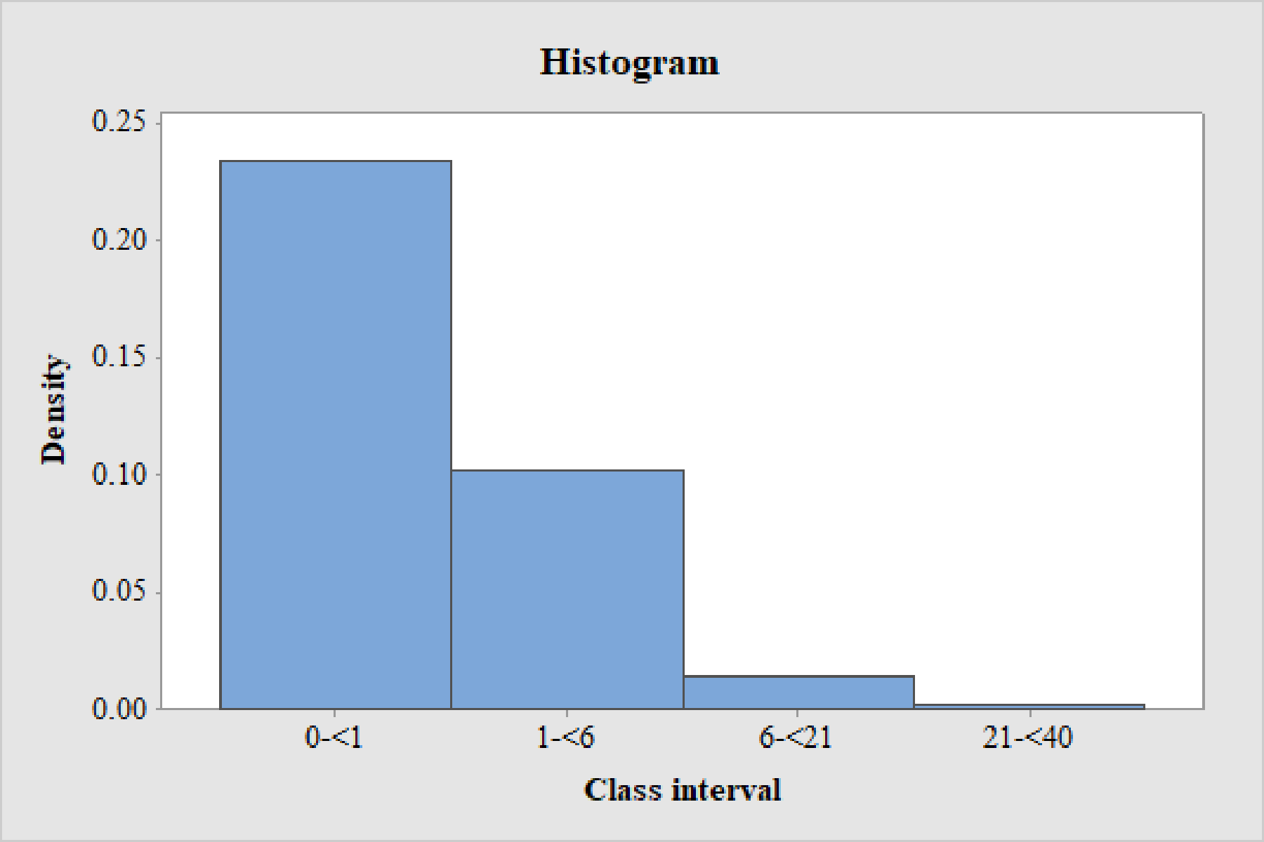
Draw the histogram for the social media data.
Answer to Problem 29E
Output using MINITAB is given below.
Explanation of Solution
Calculation:
The data represents the relative frequency distribution for the number of hours spent online at social network by students at four year colleges. The maximum value is given as 40.
For the continuous data with unequal class width, the vertical scale of the histogram must be density scale. The rectangle heights are the densities of the intervals.
Here, the class intervals do not have equal length. Hence, the histogram with the relative frequencies is not appropriate.
Therefore, the density of the data has to be used to draw a histogram.
The general formula for the rectangle height or density is,
Densities of class intervals:
Substitute the relative frequency of the class interval 0-<1 as “0.234”.
Substitute class width as,
Therefore, the density of the class intervals 0-<1 is,
Similarly, densities for the remaining class intervals are obtained below:
| Class interval | Relative frequency | Class width | Density |
| 0-<1 | 0.234 | ||
| 1-<6 | 0.512 | ||
| 6-<21 | 0.211 | ||
| 21-<40 | 0.044 |
Histogram:
Software procedure:
Step by step procedure to draw the histogram using MINITAB software.
- Select Graph > Bar chart.
- In Bars represent select values from a table.
- In one column of values select Simple.
- Enter density in Graph variables.
- Enter Class interval in categorical variable.
- In gap between clusters enter 0.
- Select OK.
Observation:
From the histogram, it is observed that the distribution of number of hours spent online at social network is positively skewed with single mode.
b.
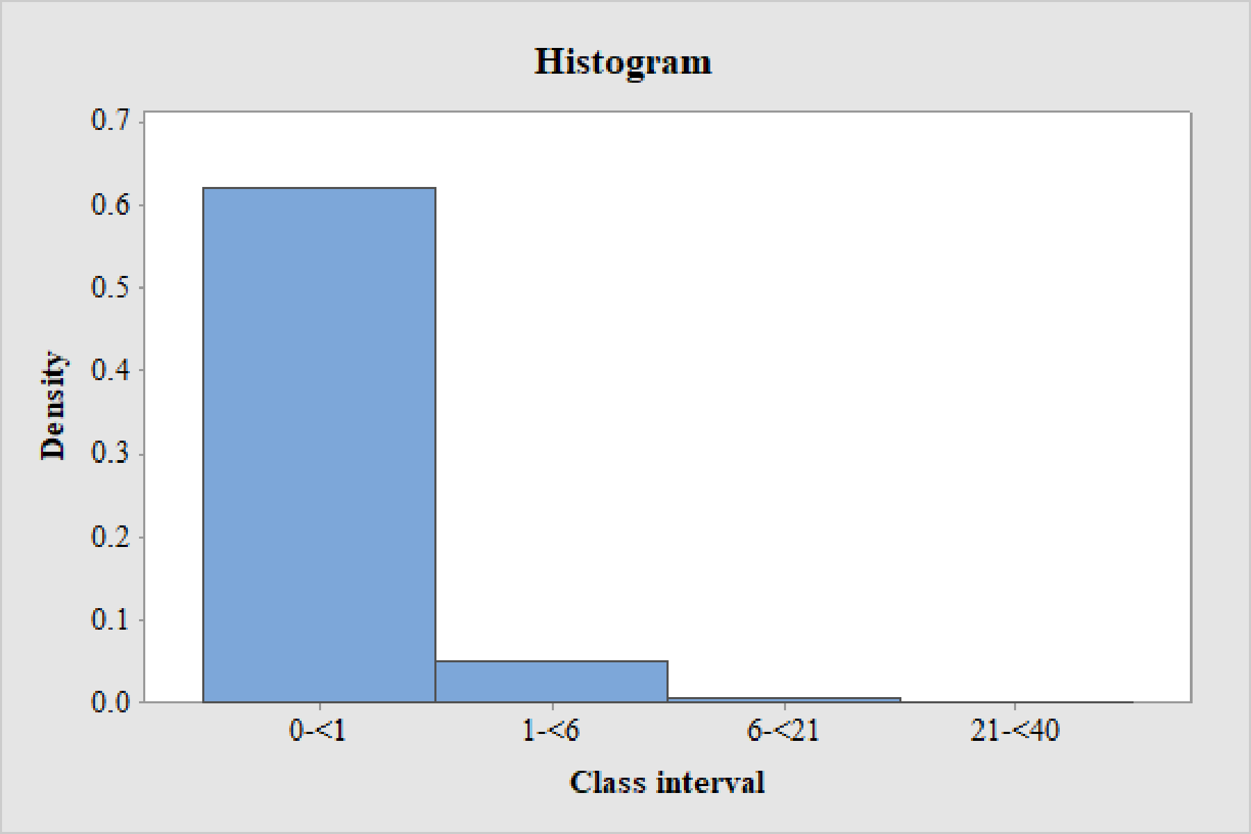
Draw the histogram for the video and computer games data.
Answer to Problem 29E
Output using MINITAB is given below.
Explanation of Solution
Calculation:
The data represents the relative frequency distribution for the number of hours spent playing video and computer games in a typical week by students at four year colleges.
For the continuous data with unequal class width, the vertical scale of the histogram must be density scale. The rectangle heights are the densities of the intervals.
Here, the class intervals do not have equal length. Hence, the histogram with the relative frequencies is not appropriate.
Therefore, the density of the angry intensity tantrum has to be used to draw a histogram.
The general formula for the rectangle height or density is,
Densities of class intervals:
Substitute the relative frequency of the class interval 0-<1 as “0.234”.
Substitute class width as,
Therefore, density of the class intervals 0-<1 is,
Similarly, densities for the remaining class intervals are obtained below:
| Class interval | Relative frequency | Class width | Density |
| 0-<1 | 0.621 | ||
| 1-<6 | 0.252 | ||
| 6-<21 | 0.108 | ||
| 21-<40 | 0.020 |
Histogram:
Software procedure:
Step by step procedure to draw the histogram using MINITAB software.
- Select Graph > Bar chart.
- In Bars represent select values from a table.
- In one column of values select Simple.
- Enter density in Graph variables.
- Enter Class interval in categorical variable.
- In gap between clusters enter 0.
- Select OK.
Observation:
From the histogram, it is observed that the distribution of number of hours spent playing video and computer games is positively skewed with single mode.
c.
Describe the similarities and differences between the histograms obtained in part (a) and part (b).
Explanation of Solution
The following similarities and differences are observed between the two histograms:
- Since, the right tail of the histogram obtained in part (a) is longer than the right tail of the histogram obtained in part (b), it can be said that students spent longer time on social media than on games.
- Both the distributions of “number of hours spent online at social network” and “number of hours spent playing video and computer games” are positively skewed with single mode.
- The variability in number of hours spent online at social network higher than the variability in number of hours spent playing video and computer games.
Want to see more full solutions like this?
Chapter 3 Solutions
Introduction To Statistics And Data Analysis
Additional Math Textbook Solutions
Statistical Techniques in Business and Economics
Fundamentals of Statistics (5th Edition)
Elementary Statistics: A Step By Step Approach
Statistics Through Applications
Statistics for Business and Economics (13th Edition)
STATISTICS F/BUSINESS+ECONOMICS-TEXT


 Glencoe Algebra 1, Student Edition, 9780079039897...AlgebraISBN:9780079039897Author:CarterPublisher:McGraw Hill
 Holt Mcdougal Larson Pre-algebra: Student Edition...AlgebraISBN:9780547587776Author:HOLT MCDOUGALPublisher:HOLT MCDOUGAL