Concept explainers
Videos
In Problems 9-14,
(a) Draw a
(b) Find
(c) Find the sample
Marketing: Coupons Each box of Healthy Crunch breakfast cereal contains a coupon entitling you to a free package of garden seeds. At the Healthy Crunch home office, they use the weight of incoming mail to determine how many of their employees are to be assigned to collecting coupons and mailing out seed packages on a given day. (Healthy Crunch has a policy of answering all its mail on the day it is received.)
Let x = weight of incoming mail and y = number of employees required to process the mail in one working day. A random sample of 8 days gave the following data:
| x(lb) | 11 | 20 | 16 | 6 | 12 18 23 | 25 |
| y (Number of employees) | 6 | 10 | 9 | 5 | 8 14 13 | 16 |
Complete parts (a) through (c), given
(d) If Healthy Crunch receives 15 pounds of mail, how many employees should be assigned mail duty that day?
(a)
To graph: The scatter diagram.
Explanation of Solution
Given: The data which consists of variables, ‘weight of incoming mail in pounds’ and ‘number of employess required to process the mail in 1 working day’, represented by x and y, respectively, is provided.
Graph:
Follow the steps given below in Excel to obtain the scatter diagram of the data.
Step 1: Enter the data into Excel sheet. The screenshot is given below.
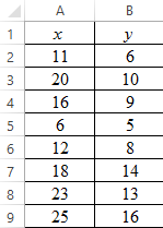
Step 2: Select the data and click on ‘Insert’. Go to charts and select the chart type ‘Scatter’.
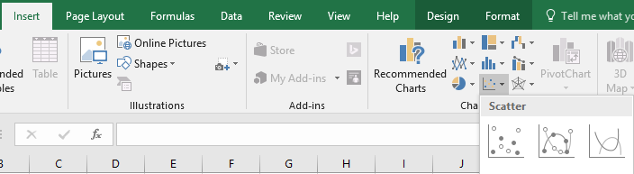
Step 3: Select the first plot and then click ‘add chart element’ provided on the left corner of the menu bar. Insert the ‘Axis titles’ and ‘Chart title’. The scatter plot for the provided data is shown below:
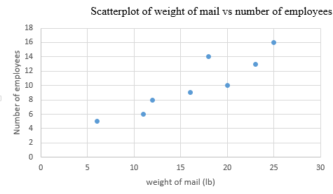
Interpretation: The scatter plot shows that there is a high positive correlation between the weight of mail and the number of employees required to process the mail.
(b)
To find: The values of
Answer to Problem 13CR
Solution: The calculated values are
Explanation of Solution
Given: The provided values are
Calculation:
The value of
The value of
The value of
Therefore, the values are
The general formula for the least-squares line is,
Here, a is the y-intercept and b is the slope.
The value of
Substitute the values of a and b in the general equation to get the least-squares line of the data. That is,
Therefore, the least-squares line is
Follow the steps given below in Excel to obtain the least-squares line on the scatter diagram.
Step 1: Enter the data into Excel sheet. The screenshot is given below.
Step 2: Select the data and click on ‘Insert’. Go to charts and select the chart type ‘Scatter’.
Step 3: Select the first plot and then click ‘add chart element’ provided in the left corner of the menu bar. Insert the ‘Axis titles’ and ‘Chart title’. The scatter plot for the provided data is shown below:
Step 4: Right click on any data point and select ‘Add Trend line’. A dialogue box will appear then select ‘linear’ and check ‘Display Equation on Chart’.
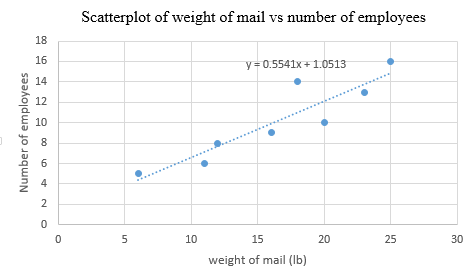
Interpretation: The scatter plot displays the equation of the least-squares line,
(c)
The values of r and
Answer to Problem 13CR
Solution: The values of r and
Explanation of Solution
Given: The provided values are
Calculation: The value of
Substitute the values in the above formula. Thus,
The coefficient of determination
Therefore, the value of
The value of
Interpretation: The correlation coefficient value
(d)
To find: The least-squares line forecast for y at
Answer to Problem 13CR
Solution: The forecasted value is about 9.
Explanation of Solution
Given: The least-squares line from part (b) is
Calculation:
The predicted value
Thus, the value of
Interpretation: If Healthy Crunch receives 15 pounds of mail, it is predicted using the least-squares line that about 9 employees should be assigned mail duty for a day.
Want to see more full solutions like this?
Chapter 4 Solutions
Understanding Basic Statistics


 MATLAB: An Introduction with ApplicationsStatisticsISBN:9781119256830Author:Amos GilatPublisher:John Wiley & Sons Inc
 Probability and Statistics for Engineering and th...StatisticsISBN:9781305251809Author:Jay L. DevorePublisher:Cengage Learning
 Statistics for The Behavioral Sciences (MindTap C...StatisticsISBN:9781305504912Author:Frederick J Gravetter, Larry B. WallnauPublisher:Cengage Learning
 Elementary Statistics: Picturing the World (7th E...StatisticsISBN:9780134683416Author:Ron Larson, Betsy FarberPublisher:PEARSON
 The Basic Practice of StatisticsStatisticsISBN:9781319042578Author:David S. Moore, William I. Notz, Michael A. FlignerPublisher:W. H. Freeman
 Introduction to the Practice of StatisticsStatisticsISBN:9781319013387Author:David S. Moore, George P. McCabe, Bruce A. CraigPublisher:W. H. Freeman