Concept explainers
Videos
Consider steady, incompressible, two-dimensional shear flow for which the velocity field is
(a) In similar fashion, calculate the location of each of the other three corners of the fluid particle at time t+dt.
(b) From the fundamental definition of linear strain rate (the rate of increase in length per unit length), calculate linear strain rates
(c) Compare your results with those obtained from the equations for
(a)
The location of each of the other three corners of the fluid particle at time
Answer to Problem 66P
The location of the lower left corner after time
The location of the lower right corner after time
The location of the upper left corner after time
The location of the upper right corner after time
Explanation of Solution
Given information:
Two-dimensional shear flow, flow is incompressible, the velocity field is
Write the expression for the two-dimensional velocity field in the vector form.
Here, the constants are
The following figure shows the position of the corners at time
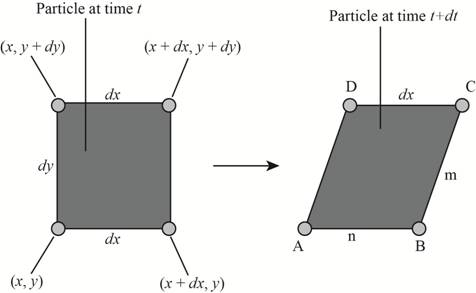
Figure-(1)
Here, the length of the lower edge at time
Write the expression for location of the lower left corner after time
Write the expression for location of the lower right corner after time
Write the expression for location of the upper left corner after time
Write the expression for location of the upper right corner after time
Write the expression for velocity along x direction.
Calculation:
Substitute
Substitute
Substitute
Substitute
Conclusion:
The location of the lower left corner after time
The location of the lower right corner after time
The location of the upper left corner after time
The location of the upper right corner after time
(b)
The linear strain rates.
Answer to Problem 66P
The linear strain rate along x axis is
The linear strain rate along y axis is
Explanation of Solution
Write the expression for the strain rate along x direction.
Write the expression for the strain rate along y direction.
Write the expression for the length of the lower edge at time
Write the expression for the length of the lower edge at time
Calculation:
Substitute
Substitute
Substitute
Conclusion:
The linear strain rate along x axis is
The linear strain rate along y axis is
(c)
The linear strain rates in Cartesian coordinates.
Comparison of the linear strain rate by fundamental principal to the linear strain rates in Cartesian coordinates.
Answer to Problem 66P
The linear strain rate in Cartesian coordinates along x axis is
The linear strain rate in Cartesian coordinates along y axis is
The linear strain rate by fundamental principal and the linear strain rates in Cartesian coordinates are same
Explanation of Solution
Given information:
Linear strain along x axis is
Write the expression for the velocity along y direction.
Write the expression for the linear strain rate along x direction in Cartesian coordination.
Write the expression for the linear strain rate along y direction in Cartesian coordination.
Calculation:
Substitute
Substitute
Conclusion:
The linear strain rate in Cartesian coordinates along x axis is
The linear strain rate in Cartesian coordinates along y axis is
The linear strain rate by fundamental principal and the linear strain rates in Cartesian coordinates are the same.
Want to see more full solutions like this?
Chapter 4 Solutions
Fluid Mechanics: Fundamentals and Applications


- A steady, incompressible, two-dimensional velocity field is given by V-›= (u, ? ) = (2xy + 1) i-›+ (−y2 − 0.6) j-› where the x- and y-coordinates are in meters and the magnitude of velocity is in m/s. The angular velocity of this flow is (a) 0 (b) −2yk-› (c) 2yk-› (d ) −2xk-› (e) −xk-›arrow_forwardThe compressible form of the continuity equation is (∂?/∂t) + ∇-›·(?V-›) = 0. Expand this equation as far as possible in Cartesian coordinates (x, y, z) and (u, ?, w).arrow_forwardThe radial velocity component in a incomplreesible, two-dimensional steady flow field (v2=0) is in the figure. Determine the acceleration field a(->) (r,θ)arrow_forward
- The velocity field of a flow is described by V-›= (4x) i-›+ (5y + 3) j-›+ (3t2)k-›. What is the pathline of a particle at a location (1 m, 2 m, 4 m) at time t = 1 s?arrow_forwardConsider the steady, two-dimensional, incompressible velocity field, V-› = (u, ?)=(ax + b) i-› + (−ay + c) j-›, where a, b, and c are constants. Calculate the pressure as a function of x and y.arrow_forwardConsider the following steady, three-dimensional veloc ity field in Cartesian coordinates: V-› = (u, ?, w) = (axy2 − b) i-› −2cy3 j-› + dxyk →, where a, b, c, and d are constants. Under what conditions is this flow field incompressible?arrow_forward
- A steady, two-dimensional, incompressible flow field in the xy-plane has a stream function given by ? = ax2 + by2 + cy, where a, b, and c are constants. The expression for the velocity component u is (a) 2ax (b) 2by + c (c) −2ax (d ) −2by − c (e) 2ax + 2by + carrow_forwardConsider the following steady, three-dimensional velocity field in Cartesian coordinates: V-› = (u, ?, w) = (axz2 − by) i-› + cxyz j-› + (dz3 + exz2)k →, where a, b, c, d, and e are constants. Under what conditions is this flow field incompressible? What are the primary dimensions of constants a, b, c, d, and e?arrow_forwardconsider the 2 dimensional velocity field V= -Ayi +Axj where in this flow field does the speed equal to A? Where does the speed equal to 2A?arrow_forward
- Consider the steady, two-dimensional, incompressible velocity field, namely, V-›= (u, ?) = (ax + b) i-›+ (−ay + cx) j-›. Calculate the pressure as a function of x and y.arrow_forwardA potential steady and incompressible air flow on x-y plane has velocity in y-direction v= - 6 xy . Determine the velocity in x-direction u=? and Stream Function SF=? ( x2 : square of x ; x3: third power of x ; y2: square of y , y3: third power of y)ANSWER: u= 3 x2 - 3 y2 SF= 3 x2 y - y3arrow_forwardA solid circular cylinder of radius R rotates at angularvelocity V in a viscous incompressible fluid that is at restfar from the cylinder, as in Fig. P4.82. Make simplifyingassumptions and derive the governing differential equationand boundary conditions for the velocity field υ θ in thefluid. Do not solve unless you are obsessed with this problem.What is the steady-state flow field for this problem?arrow_forward
 Elements Of ElectromagneticsMechanical EngineeringISBN:9780190698614Author:Sadiku, Matthew N. O.Publisher:Oxford University Press
 Mechanics of Materials (10th Edition)Mechanical EngineeringISBN:9780134319650Author:Russell C. HibbelerPublisher:PEARSON
 Thermodynamics: An Engineering ApproachMechanical EngineeringISBN:9781259822674Author:Yunus A. Cengel Dr., Michael A. BolesPublisher:McGraw-Hill Education
 Control Systems EngineeringMechanical EngineeringISBN:9781118170519Author:Norman S. NisePublisher:WILEY
 Mechanics of Materials (MindTap Course List)Mechanical EngineeringISBN:9781337093347Author:Barry J. Goodno, James M. GerePublisher:Cengage Learning
 Engineering Mechanics: StaticsMechanical EngineeringISBN:9781118807330Author:James L. Meriam, L. G. Kraige, J. N. BoltonPublisher:WILEY