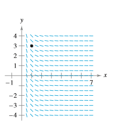
Slope Field In Exercises 45 and 46, a differential equation, a point, and a slope field are given. A slope field (or direction field) consists of line segments with slopes given by the differential equation. These line segments give a visual perspective of the slopes of the solutions of the differential equation, (a) Sketch two approximate solutions of the differential equation on the slope field, one of which passes through the indicated point. (To print an enlarged copy of the graph, go to MathGraphs.com.) (b) Use integration and the given point to find the particular solution of the differential equation and use a graphing utility to graph the solution. Compare the result with the sketch in part (a) that passes through the given point. d y d x = − 1 x 2 , x > 0 , ( 1 , 3 )
Slope Field In Exercises 45 and 46, a differential equation, a point, and a slope field are given. A slope field (or direction field) consists of line segments with slopes given by the differential equation. These line segments give a visual perspective of the slopes of the solutions of the differential equation, (a) Sketch two approximate solutions of the differential equation on the slope field, one of which passes through the indicated point. (To print an enlarged copy of the graph, go to MathGraphs.com.) (b) Use integration and the given point to find the particular solution of the differential equation and use a graphing utility to graph the solution. Compare the result with the sketch in part (a) that passes through the given point. d y d x = − 1 x 2 , x > 0 , ( 1 , 3 )
Solution Summary: The author explains how the two approximate solutions of the differential equation on the slope field can be made by using the Maple as, Interpretation: From the graph, the function behaviour remains same for different points.
Slope Field In Exercises 45 and 46, a differential equation, a point, and a slope field are given. A slope field (or direction field) consists of line segments with slopes given by the differential equation. These line segments give a visual perspective of the slopes of the solutions of the differential equation, (a) Sketch two approximate solutions of the differential equation on the slope field, one of which passes through the indicated point. (To print an enlarged copy of the graph, go to MathGraphs.com.) (b) Use integration and the given point to find the particular solution of the differential equation and use a graphing utility to graph the solution. Compare the result with the sketch in part (a) that passes through the given point.
d
y
d
x
=
−
1
x
2
,
x
>
0
,
(
1
,
3
)
With differentiation, one of the major concepts of calculus. Integration involves the calculation of an integral, which is useful to find many quantities such as areas, volumes, and displacement.
Need a deep-dive on the concept behind this application? Look no further. Learn more about this topic, calculus and related others by exploring similar questions and additional content below.
01 - What Is A Differential Equation in Calculus? Learn to Solve Ordinary Differential Equations.; Author: Math and Science;https://www.youtube.com/watch?v=K80YEHQpx9g;License: Standard YouTube License, CC-BY
Higher Order Differential Equation with constant coefficient (GATE) (Part 1) l GATE 2018; Author: GATE Lectures by Dishank;https://www.youtube.com/watch?v=ODxP7BbqAjA;License: Standard YouTube License, CC-BY


 Elementary Linear Algebra (MindTap Course List)AlgebraISBN:9781305658004Author:Ron LarsonPublisher:Cengage Learning
 Algebra & Trigonometry with Analytic GeometryAlgebraISBN:9781133382119Author:SwokowskiPublisher:Cengage
 Functions and Change: A Modeling Approach to Coll...AlgebraISBN:9781337111348Author:Bruce Crauder, Benny Evans, Alan NoellPublisher:Cengage Learning