
Introduction To Statistics And Data Analysis
6th Edition
ISBN: 9781337793612
Author: PECK, Roxy.
Publisher: Cengage Learning,
expand_more
expand_more
format_list_bulleted
Concept explainers
Videos
Textbook Question
Chapter 5.4, Problem 54E
The following data on x = Frying time (in seconds) and y = Moisture content (%) appeared in the paper “Thermal and Physical Properties of Tortilla Chips as a
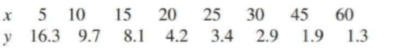
- a. Construct a scatterplot of the data.
- b. Would a line provide an effective summary of the relationship? Explain.
Expert Solution & Answer

Trending nowThis is a popular solution!

Students have asked these similar questions
A study is made of the relationship between annual production volume of Good A and factory floor area. Table below shows the data from a sample of 10 factories.
Factory
Factory floor area, X (‘000m2 )
Annual production volume, Y ($‘ 000)
1
40
3.5
2
600
25.0
3
60
4.8
4
72
3.5
5
400
30.0
6
90
5.0
7
200
12.0
8
70
4.5
9
80
5.0
10
84
6.0
Construct a scatter plot.
The following data measured the stress hormone of steelhead fish as a function of the oxygen content in the water. These data are given below:
oxygen
25
36
48
59
62
72
80
100
100
137
hormone
155
184
180
220
280
163
230
222
241
350
Construct a scatterplot and discuss its characteristics
Does there appear to be a relationship between water oxygen levels and hormone levels?
In a recent survey, ice cream truck drivers in Cincinnati, Ohio, reported that they make about $280 in income on a typical summer day. The income was generally higher on days with longer work hours, particularly hot days, and on holidays. The accompanying data file includes five weeks of the driver’s daily income (Income), number of hours on the road (Hours), whether it was a particularly hot day (Hot = 1 if the high temperature was above 85°F, 0 otherwise), and whether it was a Holiday (Holiday = 1, 0 otherwise).
Income
Hours
Hot
Holiday
196
5
1
0
282
8
0
0
318
6
1
0
232
5
1
0
276
8
0
0
312
8
0
1
193
5
0
1
110
4
0
0
321
8
1
0
283
8
0
0
325
8
1
0
247
7
0
1
398
8
1
1
448
8
1
1
214
4
0
0
235
8
0
0
238
8
0
0
148
3
1
0
313
8
0
1
449
8
1
1
332
8
1
1
247
8
0
0
363
7
1
0
393
7
1
1
254
8
0
0
228
8
0
0
355
6
1
1
248
7
0
1
291
8
1
0
255
5
1
0
239
6
0
0
181
6
0
0
222
7
0
0
170
5
0
1
374
6
1
1
1. Estimate the effect of…
Chapter 5 Solutions
Introduction To Statistics And Data Analysis
Ch. 5.1 - For each of the scatterplots shown, answer the...Ch. 5.1 - For each of the following pairs of variables,...Ch. 5.1 - For each of the following pairs of variables,...Ch. 5.1 - For each of the following pairs of variables,...Ch. 5.1 - Is the following statement correct? Explain why or...Ch. 5.1 - Draw a scatterplot for which r = 1.Ch. 5.1 - Draw a scatterplot for which r = 1.Ch. 5.1 - Each year J.D. Power and Associates surveys new...Ch. 5.1 - The accompanying data are x = Cost (cents per...Ch. 5.1 - The authors of the paper Flat-footedness Is Not a...
Ch. 5.1 - The paper The Relationship Between Cell Phone Use,...Ch. 5.1 - Data from the U.S. Federal Reserve Board (federal...Ch. 5.1 - The article 115K! The 13 Best Paying U.S....Ch. 5.1 - It may seem odd, but one of the ways biologists...Ch. 5.1 - An auction house released a list of 25 recently...Ch. 5.1 - A sample of automobiles traversing a certain...Ch. 5.2 - Two scatterplots are shown below. Explain why it...Ch. 5.2 - The authors of the paper Statistical Methods for...Ch. 5.2 - The accompanying data are a subset of data from...Ch. 5.2 - The authors of the paper Evaluating Existing...Ch. 5.2 - The authors of the paper referenced in the...Ch. 5.2 - A sample of 548 ethnically diverse students from...Ch. 5.2 - The relationship between hospital patient-to-nurse...Ch. 5.2 - The report Airline Quality Rating 2016...Ch. 5.2 - Acrylamide is a chemical that is sometimes found...Ch. 5.2 - Use the acrylamide data given in the previous...Ch. 5.2 - Studies have shown that people who suffer sudden...Ch. 5.2 - The data given in the previous exercise on x =...Ch. 5.2 - An article on the cost of housing in Califomia...Ch. 5.2 - The following data on sale price, size, and...Ch. 5.2 - Explain why it can be dangerous to use the...Ch. 5.2 - The sales manager of a large company selected a...Ch. 5.2 - Explain why the slope b of the least-squares line...Ch. 5.2 - Prob. 34ECh. 5.3 - Does it pay to stay in school? The report Trends...Ch. 5.3 - The data in the accompanying table is from the...Ch. 5.3 - The paper referenced in the previous exercise also...Ch. 5.3 - Consider the residual plot from the previous...Ch. 5.3 - The report Airline Quality Rating 2016...Ch. 5.3 - Acrylamide is a chemical that is sometimes found...Ch. 5.3 - Consider the scatterplot of acrylamide...Ch. 5.3 - Some types of algae have the potential to cause...Ch. 5.3 - The relationship between x = Total number of...Ch. 5.3 - The residuals from the least-squares line for the...Ch. 5.3 - The first Batman movie was made over 50 years ago...Ch. 5.3 - The article 115K! The 13 Best Paying U.S....Ch. 5.3 - The article Examined Life: What Stanley H. Kaplan...Ch. 5.3 - The accompanying data are a subset of data from...Ch. 5.3 - The article California State Parks Closure List...Ch. 5.3 - The article referenced in the previous exercise...Ch. 5.3 - A study was carried out to investigate the...Ch. 5.3 - Both r2 and se are used to assess the fit of a...Ch. 5.3 - Prob. 53ECh. 5.4 - The following data on x = Frying time (in seconds)...Ch. 5.4 - Use the information provided in the previous...Ch. 5.4 - The paper Aspects of Food Finding by Wintering...Ch. 5.4 - Food intake of grazing animals is limited by the...Ch. 5.4 - A study, described in the paper Prediction of...Ch. 5.4 - Prob. 59ECh. 5.4 - The following table gives the number of heart...Ch. 5.4 - Refer to the heart transplant data given in the...Ch. 5.4 - The paper Population Pressure and Agricultural...Ch. 5.4 - Determining the age of an animal can sometimes be...Ch. 5.5 - The paper How Lead Exposure Relates to Temporal...Ch. 5.5 - The following quote is from the paper Evaluation...Ch. 5 - The accompanying data represent x = Amount of...Ch. 5 - The paper A Cross-National Relationship Between...Ch. 5 - The following data on x = Score on a measure of...Ch. 5 - The paper Effects of Canine Parvovirus (CPV) on...Ch. 5 - The paper Depression, Body Mass Index, and Chronic...Ch. 5 - The paper Aspects of Food Finding by Wintering...Ch. 5 - Data on salmon availability (x) and the percentage...Ch. 5 - No tortilla chip lover likes soggy chips, so it is...Ch. 5 - The article Reduction is Soluble Protein and...Ch. 5 - The following quote is from the paper The Weight...Ch. 5 - An accurate assessment of oxygen consumption...Ch. 5 - Consider the four (x, y) pairs (0, 0), (1, 1), 1,...Ch. 5 - Prob. 1CRECh. 5 - Data from a survey of 1046 adults age 50 and older...Ch. 5 - Prob. 3CRECh. 5 - Prob. 4CRECh. 5 - Prob. 5CRECh. 5 - The amount of money spent each year on science,...Ch. 5 - Below are the data used to construct the time...Ch. 5 - In August 2009, Harris Interactive released the...Ch. 5 - Prob. 9CRECh. 5 - Prob. 10CRECh. 5 - Prob. 11CRECh. 5 - Prob. 12CRECh. 5 - Cost-to-charge ratios (the percentage of the...Ch. 5 - In the article Reproductive Biology of the Aquatic...Ch. 5 - Prob. 15CRECh. 5 - Anabolic steroid abuse has been increasing despite...Ch. 5 - Prob. 81ECh. 5 - Prob. 82ECh. 5 - Prob. 83ECh. 5 - Prob. 84ECh. 5 - Suppose the hypothetical data below are from a...Ch. 5 - Prob. 86E
Knowledge Booster


Learn more about
Need a deep-dive on the concept behind this application? Look no further. Learn more about this topic, statistics and related others by exploring similar questions and additional content below.Similar questions
- Consider the following data relating hours spent studying (X) and average grade on course quizzes (Y): X Y 5 6 3 8 4 8 7 10 5 7 6 9 Compute SP (equation below) 420 5 6 17arrow_forwardThe following table gives the millions of metric tons of carbon dioxide emissions in a certain country for selected years from 2010 and projected to 2032. Year 2010 2012 2014 2016 2018 2020 CO2 Emissions 337.5 361.5 395.1 425.8 451.1 496.4 Year 2022 2024 2026 2028 2030 2032 CO2 Emissions 558.2 592.9 628.7 662.1 709.1 742.7 (a) Create a linear function that models these data, with x as the number of years past 2010 and y as the millions of metric tons of carbon dioxide emissions. (Round all numerical values to two decimal places.)y(x) = (b) Find the model's estimate for the 2028 data point. (Round your answer to two decimal places.) million metric tons(c) Find the slope of the linear model. (Round your answer to two decimal places.)Interpret the slope of the linear model. For each year since ---Select--- 2009 2010 2015 2028 2032 , carbon dioxide emissions in the U.S. are expected to change by million metric tons.arrow_forwardConsider the following data relating hours spent studying (X) and average grade on course quizzes (Y): X Y 5 6 3 8 4 8 7 10 5 7 6 9 From these observations, can we conclude that hours spent studying caused increases in quiz grades?arrow_forward
- The following table shows the annual expenditures, in dollars, per customer unit for residential landline phone services and cellular phone services in the United States in the given year.† Year Landline Cell 2004 592 378 2006 542 524 2008 467 643 2010 401 760 Calculate the regression line for each type of service. (Let t be the time in years since 2004, L be the operating revenue of landline phone services and C be the expenditure of cellular services. Round your regression parameters to two decimal places.) L(t) = C(t) = Determine the expenditure level at which the two lines cross. Round your answer for the expenditure level to one decimal place. million dollarsarrow_forwardShown below is a portion of a computer output for a linear regression analysis relating an individual's income (y in thousands of dollars) to age (x1 in years), level of education (x2 ranging from 1 to 5), and the individual's gender (x3 where 0 = female and 1 = male). Coefficient Standard Error t-statistic p-value Intercept 15.934 1.389 11.47 0.000 x1 0.625 0.094 6.65 0.000 x2 0.921 0.190 4.85 0.000 x3 –0.510 0.920 –0.55 0.590 Source of Variation Sum of squares Degrees of freedom Mean square F-statistic p-value Regression 84 3 28 4 0.027 Error 112 16 7 Total 196 19 a. Is there a significant relationship between an individual's income and the set of variables, age, level of education, and gender (based on a significance level α =05 )? Explain why using one of the p-values in the output tables. b.Which of the three predictor variables are…arrow_forwardA researcher hypothesizes that in a certain country the net annual growth of private sector purchases of government bonds, B, is positively related to the nominal rate of interest on the bonds, NI, and negatively related to the rate of inflation Π: Bt = a0 + a1NIt + a2Π t + ut Note that it may be hypothesized that B depends on the real rate of interest on bonds, R, where R = NI – Π. Using a sample of 56 annual observations, s/he estimates the following equations: (1) Bt = 0.43 + 0.90NIt - 0.97Πt R21 = 0.962, SSR1 = 2.20, QRESET(F1,52) = 16.6 (3.58) (8.80) (-1.05) (2) Bt = 0.44 + 0.94Rt R22 = 0.960, SSR2 = 2.22, QRESET(F1,53) = 0.9 (9.70) (16.7) (3) Bt = 0.44 + 1.14NIt SSR3 = 9.20, QRESET(F1,53) = 59.9 (8.84) (36.1) (4) NIt = 0.08 + 0.94Πt R24 = 0.997, SSR4 = 0.18, QRESET(F1,53) = 1.4…arrow_forward
- The following data shows ages of musicians who performed at a concert. Age is a continuous variable. Calculate the Mode for the variable. 22 82 27 43 19 47 41 34 34 42 35arrow_forwardA highway department is studying the relationship between traffic flow and speed. The following model has been hypothesized: y = ?0 + ?1x + ? where y = traffic flow in vehicles per hour x = vehicle speed in miles per hour. The following data were collected during rush hour for six highways leading out of the city. Traffic Flow(y) Vehicle Speed(x) 1,254 35 1,330 40 1,228 30 1,334 45 1,351 50 1,126 25 In working further with this problem, statisticians suggested the use of the following curvilinear estimated regression equation. ŷ = b0 + b1x + b2x2 (a) Develop an estimated regression equation for the data of the form ŷ = b0 + b1x + b2x2. (Round b0 to the nearest integer and b1 to two decimal places and b2 to three decimal places.) ŷ = (b) Use ? = 0.01 to test for a significant relationship. Find the value of the test statistic. (Round your answer to two decimal places.) Find the p-value. (Round your answer to three decimal places.) p-value = (c)…arrow_forwardA highway department is studying the relationship between traffic flow and speed. The following model has been hypothesized: y = ?0 + ?1x + ? where y = traffic flow in vehicles per hour x = vehicle speed in miles per hour. The following data were collected during rush hour for six highways leading out of the city. Traffic Flow(y) Vehicle Speed(x) 1,254 35 1,330 40 1,228 30 1,334 45 1,351 50 1,126 25 In working further with this problem, statisticians suggested the use of the following curvilinear estimated regression equation. ŷ = b0 + b1x + b2x2 (a) Develop an estimated regression equation for the data of the form ŷ = b0 + b1x + b2x2. (Round b0 to the nearest integer and b1 to two decimal places and b2 to three decimal places.) ŷ = (b) Use ? = 0.01 to test for a significant relationship. State the null and alternative hypotheses. H0: b0 = b1 = b2 = 0Ha: One or more of the parameters is not equal to zero.H0: One or more of the parameters is…arrow_forward
- Consider the following data relating hours spent studying (X) and average grade on course quizzes (Y): X Y 5 6 3 8 4 8 7 10 5 7 6 9 Compute SSX 10 30 5 44arrow_forwardThe following table shows the annual number of PhD graduates in a country in various fields. Natural Sciences Engineering Social Sciences Education 1990 70 10 50 30 1995 130 40 100 40 2000 330 130 280 130 2005 490 370 470 210 2010 590 550 830 520 2012 690 590 1,000 900 (a) Use technology to obtain the regression equation and the coefficient of correlation r for the number of social science doctorates as a function of time t in years since 1990. (Round coefficients to three significant digits. Round your r-value to three decimal places.) y(t) = r =arrow_forwardA number of studies have shown lichens (certain plants composed of an alga and a fungus) to be excellent bioindicators of air pollution. The article “The Epiphytic Lichen Hypogymnia physodes as a Biomonitor of Atmospheric Nitrogen and Sulphur Deposition in Norway” (Environ. Monitoring Assessment, 1993: 27–47) gives the following data (read from a graph) on x ¼ NO3 wet deposition (g N/m2 ) and y ¼ lichen N (% dry weight): (refer to chart) The author used simple linear regression to analyze the data. Use the accompanying MINITAB output to answer the following questions: a. What are the least squares estimates of b0 and b1? b. Predict lichen N for an NO3 deposition value of .5. c. What is the estimate of s? d. What is the value of total variation, and how much of it can be explained by the model relationship?arrow_forward
arrow_back_ios
SEE MORE QUESTIONS
arrow_forward_ios
Recommended textbooks for you
 Algebra & Trigonometry with Analytic GeometryAlgebraISBN:9781133382119Author:SwokowskiPublisher:Cengage
Algebra & Trigonometry with Analytic Geometry
Algebra
ISBN:9781133382119
Author:Swokowski
Publisher:Cengage
Correlation Vs Regression: Difference Between them with definition & Comparison Chart; Author: Key Differences;https://www.youtube.com/watch?v=Ou2QGSJVd0U;License: Standard YouTube License, CC-BY
Correlation and Regression: Concepts with Illustrative examples; Author: LEARN & APPLY : Lean and Six Sigma;https://www.youtube.com/watch?v=xTpHD5WLuoA;License: Standard YouTube License, CC-BY