
Videos
The paper “How Lead Exposure Relates to Temporal Changes in IQ, Violent Crime, and Unwed Pregnancy” (Environmental Research [2000]: 1–22) investigated whether childhood lead exposure is related to criminal behavior in young adults. Using historical data, the author paired y = Assault rate (assaults per 100,000 people) for each year from 1964 to 1997 with a measure of lead exposure (tons of gasoline lead per 1000 people) 23 years earlier. For example, the lead exposure from 1974 was paired with the assault rate from 1997.
The author chose to go back 23 years for lead exposure because the highest number of assaults are committed by people in their early twenties, and 23 years earlier would represent a time when those in this age group were infants.
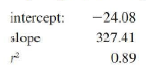
A least-squares line was used to describe the relationship between assault rate and lead exposure 23 years prior. Summary statistics given in the paper are
Use the information provided to answer the following questions.
- a. What is the value of the
correlation coefficient for x = Lead exposure 23 years prior and y = Assault rate? Interpret this value. Is it reasonable to conclude that increased lead exposure is the cause of increased assault rates? Explain. - b. What is the equation of the least-squares line? Use the line to predict assault rate in a year in which gasoline lead exposure 23 years prior was 0.5 tons per 1000 people.
- c. What proportion of year-to-year variability in assault rates can be explained by the relationship between assault rate and gasoline lead exposure 23 years earlier?
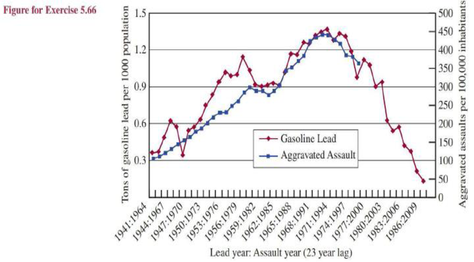
- d. The graph in the figure on the next page appeared in the paper. Note that this is not a scatterplot of the (x, y) pairs—it is two separate time series plots. The time scale 1941, 1942, ..., 1986 is the time scale used for the lead exposure data and the time scale 1964, 1965, ..., 2009 is used for the assault rate data. Also note that at the time the graph was constructed, assault rate data was only available through 1997. Spend a few minutes thinking about the information contained in this graph and then briefly explain what aspect of this graph accounts for the reported
positive correlation between assault rate and lead exposure 23 years prior.
Want to see the full answer?
Check out a sample textbook solution
Chapter 5 Solutions
Introduction To Statistics And Data Analysis


- Urban Travel Times Population of cities and driving times are related, as shown in the accompanying table, which shows the 1960 population N, in thousands, for several cities, together with the average time T, in minutes, sent by residents driving to work. City Population N Driving time T Los Angeles 6489 16.8 Pittsburgh 1804 12.6 Washington 1808 14.3 Hutchinson 38 6.1 Nashville 347 10.8 Tallahassee 48 7.3 An analysis of these data, along with data from 17 other cities in the United States and Canada, led to a power model of average driving time as a function of population. a Construct a power model of driving time in minutes as a function of population measured in thousands b Is average driving time in Pittsburgh more or less than would be expected from its population? c If you wish to move to a smaller city to reduce your average driving time to work by 25, how much smaller should the city be?arrow_forwardA paper investigated the driving behavior of teenagers by observing their vehicles as they left a high school parking lot and then again at a site approximately 1 2 mile from the school. Assume that it is reasonable to regard the teen drivers in this study as representative of the population of teen drivers. Amount by Which Speed Limit Was Exceeded MaleDriver FemaleDriver 1.2 -0.1 1.4 0.4 0.9 1.1 2.1 0.7 0.7 1.1 1.3 1.2 3 0.1 1.3 0.9 0.6 0.5 2.1 0.5 (a) Use a .01 level of significance for any hypothesis tests. Data consistent with summary quantities appearing in the paper are given in the table. The measurements represent the difference between the observed vehicle speed and the posted speed limit (in miles per hour) for a sample of male teenage drivers and a sample of female teenage drivers. (Use μmales − μfemales.Round your test statistic to two decimal places. Round your degrees of freedom down to the nearest whole number. Round your p-value to…arrow_forwardIn a study attempting to replicate findings by Stephens, Atkins, & Kingston (2009), each participant was asked to plunge a hand into the icy water and keep it there as long as the pain would allow. In one condition, the participants repeated their favorite curse words while their hands were in the water. In the other condition, they repeated neutral words. The original research showed that, in addition to lowering the participants’ perception of pain, swearing also increased the amount of time they were able to tolerate the pain. Data similar to the results obtained in the study are shown in the following table: _____________Amount of Time (in Seconds)_ Participant Swear Words Neutral Words 1 94 59 2 70 61 3 52 47 4…arrow_forward
- In a study attempting to replicate findings by Stephens, Atkins, & Kingston (2009), each participant was asked to plunge a hand into the icy water and keep it there as long as the pain would allow. In one condition, the participants repeated their favorite curse words while their hands were in the water. In the other condition, they repeated neutral words. The original research showed that, in addition to lowering the participants’ perception of pain, swearing also increased the amount of time they were able to tolerate the pain. Data similar to the results obtained in the study are shown in the following table: _____________Amount of Time (in Seconds)_ Participant Swear Words Neutral Words 1 94 59 2 70 61 3 52 47 4…arrow_forwardSuppose the marketing research firm would like to examine if the social networking site that a person primarily uses is influenced by his or her age. In a randomly drawn sample, 369 social network users were asked which site they primarily visited. At the 0.05 level of significance, can we conclude that the two variables are related? These data are presented in the following table along with each person’s age group: Age (Years) Facebook Twitter LinkedIn 10-17 7 22 0 18-34 44 54 25 35-54 40 38 44 55 and older 26 38 31 a. What test should you run? b. Select the correct hypothesis statements. H0: H1: c. Compute the value of the test statistic? (Round your answer to 2 decimal places. Negative values should have a minus sign in front of them) d. Determine the p-value (Round your final answer to 4 decimal places.) e. What is your decision regarding the null hypothesis? multiple choice Fail to reject the null. Reject the…arrow_forwardThe regional transit authority for a major metropolitan area wants to determine whether there is any relationship between the age of a bus and the annual maintenance cost. A sample of 10 buses resulted in the data in Worksheet 2. Worksheet 2 Age of a Bus (years) Maintenance Cost ($) 1 350 2 370 2 480 2 520 2 590 3 550 4 750 4 800 5 790 5 950 At the 0.05 level of significance, is there evidence of a linear relationship between the age of a bus and the annual maintenance cost.arrow_forward
- A research was conducted which revealed that the students’ usage of mobile phones has nowadays increased after the pandemic due to online classes and submission of their assignments and quizzes. Already the usage of mobile phones for the students was growing due to social media and different online games. The data of 25 students is provided to you in Table 2.1 that displays hours (time) spend by the children on mobile phones per week. Table 2.1 67 64 59 66 59 68 64 61 65 67 67 67 63 59 65 69 62 70 70 60 59 65 66 69 67 You are required to Compute the Frequency Distribution, Cumulative Frequency and Cumulative Relative Frequency. Sketch Histogram in Excel. Define the skewness of the drawn Histogram.arrow_forwardWhat is the step-step solution to this problem? Does posting calorie content for menu items affect people’s choices in fast-food restaurants? According to results obtained by Elbel, Gyamfi, and Kersh (2011), the answer is no. The researchers monitored the calorie content of food purchases for children and adolescents in four large fast-food chains before and after mandatory labeling began in New York City. Although most of the adolescents reported noticing the calorie labels, apparently the labels had no effect on their choices. Data similar to the results obtained show an average of M = 786 calories per meal with s = 85 for n = 100 children and adolescents before the labeling, compared to an average of M = 772 calories with s = 91 for a similar sample of n = 100 after the mandatory posting. Use a two-tailed test with a α .05 to determine whether the mean number of calories after the posting is significantly different than before calorie content was posted. 3. Calculate r 2 to…arrow_forwardA paper investigated the driving behavior of teenagers by observing their vehicles as they left a high school parking lot and then again at a site approximately 1 2 mile from the school. Assume that it is reasonable to regard the teen drivers in this study as representative of the population of teen drivers. MaleDriver FemaleDriver 1.4 -0.2 1.2 0.5 0.9 1.1 2.1 0.7 0.7 1.1 1.3 1.2 3 0.1 1.3 0.9 0.6 0.5 2.1 0.5 (a) Use a .01 level of significance for any hypothesis tests. Data consistent with summary quantities appearing in the paper are given in the table. The measurements represent the difference between the observed vehicle speed and the posted speed limit (in miles per hour) for a sample of male teenage drivers and a sample of female teenage drivers. (Use ?males − ?females. Round your test statistic to two decimal places. Round your degrees of freedom down to the nearest whole number. Round your p-value to three decimal places.) t = df =…arrow_forward
 Functions and Change: A Modeling Approach to Coll...AlgebraISBN:9781337111348Author:Bruce Crauder, Benny Evans, Alan NoellPublisher:Cengage Learning
 Big Ideas Math A Bridge To Success Algebra 1: Stu...AlgebraISBN:9781680331141Author:HOUGHTON MIFFLIN HARCOURTPublisher:Houghton Mifflin Harcourt