
Videos
Since laboratory or field experiments are generally expensive and time consuming,
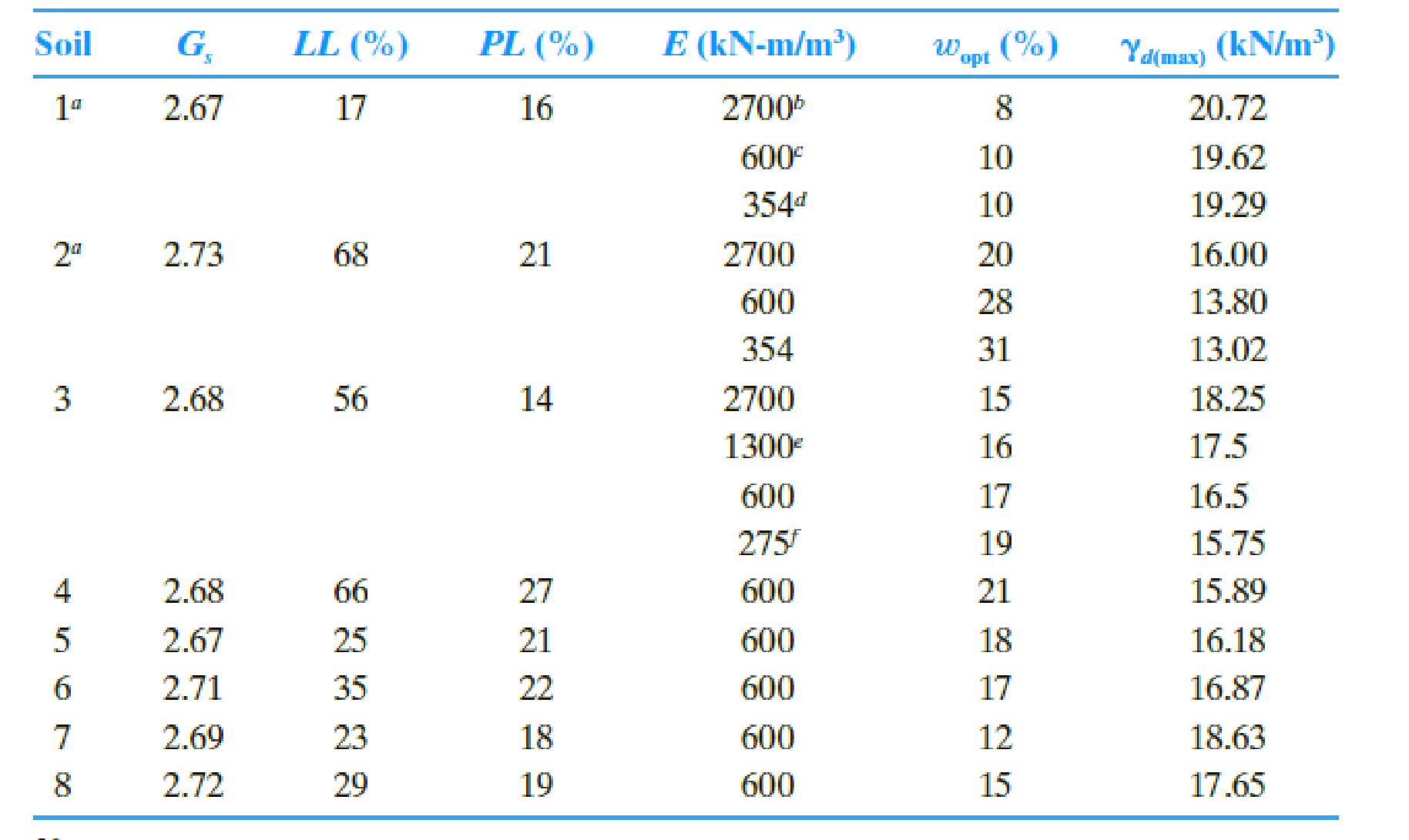
- a. Use the Osman et al. (2008) method [Eqs. (6.15) through (6.18)].
- b. Use the Gurtug and Sridharan (2004) method [Eqs. (6.13) and (6.14)].
- c. Use the Matteo et al. (2009) method [Eqs. (6.19) and (6.20)].
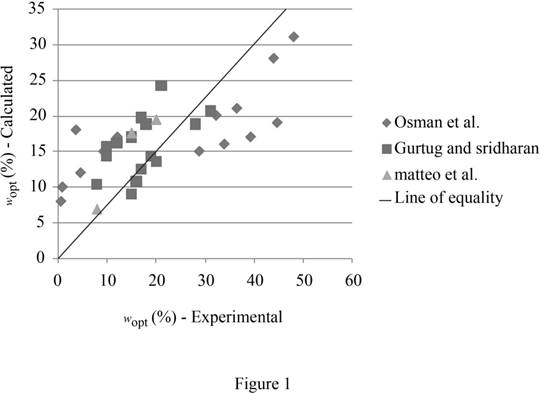
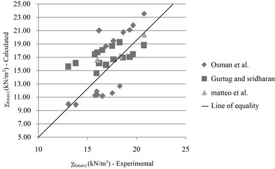
- d. Plot the calculated wopt against the experimental wopt, and the calculated γd(max) with the experimental γd(max). Draw a 45° line of equality on each plot.
- e. Comment on the predictive capabilities of various methods. What can you say about the inherent nature of empirical models?
(a)
Find the optimum moisture content and maximum dry unit weight using Osman et al. (2008) method.
Explanation of Solution
Calculation:
Determine the plasticity index PI using the relation.
Here, LL is the liquid limit for soil 1 and PL is the plastic limit for soil 1.
Substitute 17 % for LL and 16 % for PL.
Similarly, calculate the PI for remaining soils.
Determine the optimum moisture content for soil 1 using the relation.
Here, E is the compaction energy for soil 1.
Substitute
Similarly, calculate the optimum moisture content for remaining soils.
Determine the value of L using the relation.
Substitute
Determine the value of M using the relation.
Substitute
Determine the maximum dry unit weight of the soil 1 using the relation.
Substitute 23.78 for L, 0.387 for M, and 0.69 % for
Similarly, calculate the maximum dry unit weight for remaining soils.
Summarize the calculated values as in Table 1.
| Soil |
LL (%) |
PL (%) |
PI (%) |
E |
(Exp) |
(Exp) |
| L | M |
|
| 1 | 17 | 16 | 1 | 2,700 | 8 | 20.72 | 0.69 | 23.782 | 0.387 | 23.51 |
| 600 | 10 | 19.62 | 0.93 | 21.984 | 0.277 | 21.73 | ||||
| 354 | 10 | 19.29 | 1.02 | 21.354 | 0.238 | 21.11 | ||||
| 2 | 68 | 21 | 47 | 2,700 | 20 | 16.00 | 32.26 | 23.782 | 0.387 | 11.30 |
| 600 | 28 | 13.80 | 43.92 | 21.984 | 0.277 | 9.82 | ||||
| 354 | 31 | 13.02 | 48.01 | 21.354 | 0.238 | 9.91 | ||||
| 3 | 56 | 14 | 42 | 2,700 | 15 | 18.25 | 28.82 | 23.782 | 0.387 | 12.63 |
| 1,300 | 16 | 17.50 | 33.89 | 22.908 | 0.333 | 11.61 | ||||
| 600 | 17 | 16.50 | 39.24 | 21.984 | 0.277 | 11.12 | ||||
| 275 | 19 | 15.75 | 44.65 | 21.052 | 0.220 | 11.23 | ||||
| 4 | 66 | 27 | 39 | 600 | 21 | 15.89 | 36.45 | 21.984 | 0.277 | 11.89 |
| 5 | 25 | 21 | 4 | 600 | 18 | 16.18 | 3.740 | 21.984 | 0.277 | 20.95 |
| 6 | 35 | 22 | 13 | 600 | 17 | 16.87 | 12.15 | 21.984 | 0.277 | 18.62 |
| 7 | 23 | 18 | 5 | 600 | 12 | 18.63 | 4.67 | 21.984 | 0.277 | 20.69 |
| 8 | 29 | 19 | 10 | 600 | 15 | 17.65 | 9.35 | 21.984 | 0.277 | 19.39 |
(b)
Find the optimum moisture content and maximum dry unit weight using Gurtug and Sridharan (2004) method.
Explanation of Solution
Calculation:
Determine the optimum moisture content for soil 1 using the relation.
Substitute
Determine the maximum dry unit weight of the soil 1 using the relation.
Substitute 10.34 % for
Similarly, calculate the maximum dry unit weight for remaining soils.
Summarize the calculated values as in Table 2.
| Soil |
PL (%) |
E |
(Exp) |
(Exp) |
|
|
| 1 | 16 | 2,700 | 8 | 20.72 | 10.34 | 18.77 |
| 600 | 10 | 19.62 | 14.31 | 17.46 | ||
| 354 | 10 | 19.29 | 15.70 | 17.02 | ||
| 2 | 21 | 2,700 | 20 | 16.00 | 13.57 | 17.69 |
| 600 | 28 | 13.80 | 18.78 | 16.08 | ||
| 354 | 31 | 13.02 | 20.61 | 15.55 | ||
| 3 | 14 | 2,700 | 15 | 18.25 | 9.05 | 19.22 |
| 1,300 | 16 | 17.50 | 10.73 | 18.64 | ||
| 600 | 17 | 16.50 | 12.52 | 18.04 | ||
| 275 | 19 | 15.75 | 14.32 | 17.45 | ||
| 4 | 27 | 600 | 21 | 15.89 | 24.15 | 14.58 |
| 5 | 21 | 600 | 18 | 16.18 | 18.78 | 16.08 |
| 6 | 22 | 600 | 17 | 16.87 | 19.67 | 15.82 |
| 7 | 18 | 600 | 12 | 18.63 | 16.10 | 16.89 |
| 8 | 19 | 600 | 15 | 17.65 | 16.99 | 16.62 |
(c)
Find the optimum moisture content and maximum dry unit weight using Matteo et al. method.
Explanation of Solution
Calculation:
Determine the optimum moisture content for soil 1 using the relation.
Substitute 17 % LL and
Determine the maximum dry unit weight of the soil 1 using the relation.
Substitute 6.94 % for
Similarly, calculate the maximum dry unit weight for remaining soils.
Summarize the calculated values as in Table 3.
| Soil |
Specific gravity |
PI (%) |
(Exp) |
(Exp) |
|
|
| 1 | 2.67 | 1 | 8 | 20.72 | 6.94 | 20.37 |
| 10 | 19.62 | 6.94 | 20.37 | |||
| 10 | 19.29 | 6.94 | 20.37 | |||
| 2 | 2.73 | 47 | 20 | 16.00 | 19.44 | 16.60 |
| 28 | 13.80 | 19.44 | 16.60 | |||
| 31 | 13.02 | 19.44 | 16.60 | |||
| 3 | 2.68 | 42 | 15 | 18.25 | 17.56 | 17.11 |
| 16 | 17.50 | 17.56 | 17.11 | |||
| 17 | 16.50 | 17.56 | 17.11 | |||
| 19 | 15.75 | 17.56 | 17.11 | |||
| 4 | 2.68 | 39 | 21 | 15.89 | 20.31 | 16.25 |
| 5 | 2.67 | 4 | 18 | 16.18 | 9.16 | 19.52 |
| 6 | 2.71 | 13 | 17 | 16.87 | 11.36 | 18.97 |
| 7 | 2.69 | 5 | 12 | 18.63 | 8.41 | 20.25 |
| 8 | 2.72 | 10 | 15 | 17.65 | 9.67 | 19.82 |
(d)
Plot the graph between the calculated
Explanation of Solution
Refer Table 1, 2, and 3.
Draw the graph between the calculated
Draw the graph between calculated
(e)
Comment on the predictive capabilities of various methods and comment about the inherent nature of empirical models.
Explanation of Solution
Prediction of optimum moisture content:
Refer Figure (1), several data points are closely packed around the
Prediction of maximum dry unit weight:
Most data points for all models show good covenant between the calculated and the experimental values.
The empirical models are often limited to the materials, test methods and environmental conditions under which the experiments were conducted and the developed models. For new materials and conditions, the predicted values may not be reliable.
Want to see more full solutions like this?
Chapter 6 Solutions
Principles of Geotechnical Engineering (MindTap Course List)


- Repeat Problem 2.11 with the following data. 2.11 The grain-size characteristics of a soil are given in the following table. a. Draw the grain-size distribution curve. b. Determine the percentages of gravel, sand, silt, and clay according to the MIT system. c. Repeat Part b using the USDA system. d. Repeat Part b using the AASHTO system.arrow_forwardRepeat Problem 2.8 using the following data. 2.8 The following are the results of a sieve and hydrometer analysis. a. Draw the grain-size distribution curve. b. Determine the percentages of gravel, sand, silt and clay according to the MIT system. c. Repeat Part b according to the USDA system. d. Repeat Part b according to the AASHTO system.arrow_forward12. Situation 12 - The given data shows the sieve analysis of three soil samples. a. Compute for the group index of Soil B. b Compute for the group index of Soil A. c. Compute for the group index of Soil Carrow_forward
- Geotechnical laboratory tests were conducted to determine the liquid limit of soils. The data set shown in Table1 was obtained by using Casagrande's apparatus on Soil A (Plastic Limit = 32). The data set shown in Table 2was obtained by using Cone penetrometer on a different Soil B (Plastic Limit = 28).Table 1. Data from LL cup testing Table 2. Data from Cone penetrometer(a) Draw the Flow curve for soil A and B.(b) Calculate the Flow Index for both soils.(c) Calculate the Liquid limit for both soils.(d) Calculate the Plasticity and the Liquidity Indices for both soils, if both soils were found to havethe same current water content of 30%.(e) What can be said about the strengths of the soils in their current state?arrow_forwardThree kinds of experiments for measuring soil permeability coefficientarrow_forwardExplain in detail Maximum Dry Density and Optimum Moisture Content of soil? Explain in 5 sentences how you are going to interpret the results of Proctor’s Compaction test?arrow_forward
- Why do we have to trim the soil sample in undisturbed soil carefully using the soil lathe? What are the different laboratory tests for undisturbed soil sample? List them.arrow_forwardFALLING HEAD PERMEABILITY TEST OTHER QUESTIONS: 1. What is the importance of finding the coefficient of permeability of soils? 2. What is the difference between constant head permeability test and falling head permeability test? 3. Why is it needed to fully saturate the soil first before conducting the experiment? 4. Why is there a need to remove air bubbles from the specimen?arrow_forwardThe given data shows the sieve analysis of three soil samples. Compute for the group index of Soil A, B, and C.arrow_forward
- The results of standard and modified Proctor tests, along with interpretation for the curves, are given in the image below for a sandy soil being considered from a potential borrow pit for a project.Using the interpreted curve, what is the maximum dry unit weight (in pcf) of the soil for the modified Proctor test results?what is the optimum water content of the soil (in percent) for the modified Proctor test results?arrow_forwardA soil sample has the following size distribution; 4 to 2mm = 17%, 2 to 0.05 mm = 12%, 0.5 to 0.005 mm = 22% 0.005 to 0.002 mm = 10% <0.002 mm = 39% what is the percent clay silt and sand? What are the modifier and textural classification?arrow_forwardGeotechnical Engineering Please help me answer this question, and please show your solutions write it properly. Problem 4 For a given sandy soil, the maximum and minimum void ratios are 0.72 and 0.46, respectively. If Gs= 2.71 and w=11%, what is the moist unit weight of compaction in the field if the relative density equals 82%? Problem 5 A soil sample has a unit weight of 105.7 pcf and a degree of saturation of 50% When the saturation is increased to 75%, its unit weight raises to 112.7 pcf. Determine the void ratio e and the specific gravity Gs for this soil.arrow_forward
 Principles of Geotechnical Engineering (MindTap C...Civil EngineeringISBN:9781305970939Author:Braja M. Das, Khaled SobhanPublisher:Cengage Learning