Concept explainers
Videos
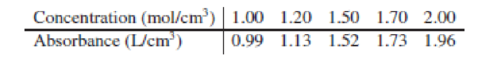
The Beer–Lambert law relates the absorbance A of a solution to the concentration C of a species in solution by A = MLC, where L is the path length and M is the molar absorption coefficient. Assume that L = 1 cm. Measurements of A are made at various concentrations. The data are presented in the following table.
- a. Let
- b. What value does the Beer–Lambert law assign to β0?
- c. What physical quantity does
- d. Test the hypothesis H0 : β0 = 0. Is the result consistent with the Beer–Lambert law?
a.
Find the values of
Answer to Problem 1SE
The values of
Explanation of Solution
Calculation:
The given information is that the Beer–Lambert law relates the absorbance A of a solution to the concentration C of a species in solution by,
Where L is the path length and M is the molar absorption coefficient.
Least-squares line:
Software Procedure:
Step-by-step procedure to obtain the least-squares line using the MINITAB software is given below:
- Choose Stat > Regression > Regression > Fit Regression Model.
- In Responses, enter “Absorbance”.
- In Continuous predictors, enter “Concentration”.
- Check Results.
- In Display of results, choose Simple tables.
- Click OK.
Output using the MINITAB software is given below:
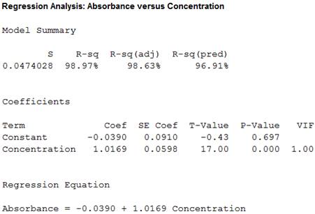
From the MINITAB output,
b.
Find the value does the Beer-Lambert law assign to
Explanation of Solution
Calculation:
Here, the variable C is independent, the variable A is dependent, the length L is constant and M is the molar absorption coefficient.
The equation of the Beer-Lambert law is,
The equation of the least-squares line for predicting absorbance (A) from concentration (C) is,
On comparing equation (1) and (2),
Thus, the coefficient
c.
Find the physical quantity does
Explanation of Solution
Justification:
From part b., comparing equation (1) and (2) is,
Therefore, the coefficient
d.
Test the hypothesis
Check whether the result is consistent with the Beer-Lambert law.
Answer to Problem 1SE
Yes, the result is consistent with the Beer-Lambert law.
Explanation of Solution
Calculation:
State the null and alternative hypotheses.
Null hypothesis:
Alternative hypothesis:
From the MINITAB obtained in part a., the test statistic for slope is –0.43 and the P- value is 0.697.
Conclusion:
Here, the P-value is not small.
That is, the P-value is greater than the level of significance, 0.05.
Therefore, the null hypothesis is not rejected.
Hence, it can be concluded that
Thus, the result is consistent with the Beer-Lambert law.
Want to see more full solutions like this?
Chapter 7 Solutions
STATISTICS FOR ENGR.+SCI.(LL)-W/ACCESS
Additional Math Textbook Solutions
Elementary Statistics: Picturing the World (6th Edition)
Business Analytics
Essentials of Statistics (6th Edition)
Intro Stats, Books a la Carte Edition (5th Edition)
Statistics: Informed Decisions Using Data (5th Edition)
PRACTICE OF STATISTICS F/AP EXAM


- For some genetic mutations, it is thought that the frequency of the mutant gene in men increases linearly with age. If m1 is the frequency at age t1, and m2 is the frequency at age t2, then the yearly rate of increase is estimated by r = (m2 − m1)/(t2 − t1). In a polymerase chain reaction assay, the frequency in 20-year-old men was estimated to be 17.7 ± 1.7 per μgDNA, and the frequency in 40-year-old men was estimated to be 35.9 ± 5.8 per μg DNA. Assume that age is measured with negligible uncertainty.a) Estimate the yearly rate of increase, and find the uncertainty in the estimate.b) Find the relative uncertainty in the estimated rate of increase.arrow_forwardTable 14.17 The Least Squares Point Estimates for Exercise 14.51 Bo = 10.3676 (.3710) B1 = .0500 (<.001) B2 = 6.3218 (.0152) B3 = -11.1032 (.0635) B4 = -.4319 (.0002) Questions Using the t statistic and appropriate critical values, test Ho: βj = 0 versus Ha: βj ≠ 0 by setting α equal to .05. Which independent variables are significantly related to y in the model with α = .05? Using the t statistic and appropriate critical values, test Ho: βj = 0 versus Ha: βj ≠ 0 by setting α equal to .01. Which independent variables are significantly related to y in the model with α = .01? Find the p-value for testing Ho: βj = 0 versus Ha: βj ≠ 0 on the output. Using the p-value, determine whether we can reject Ho by setting α equal to .10, .05, .01, and .001. What do you conclude about the significance of the independent variables in the model? Calculate the 95 percent confidence interval for βj. Discuss one practical application of this interval. Calculate the 99 percent confidence interval for…arrow_forwardIn a typical multiple linear regression model where x1 and x2 are non-random regressors, the expected value of the response variable y given x1 and x2 is denoted by E(y | 2,, X2). Build a multiple linear regression model for E (y | *,, *2) such that the value of E(y | x1, X2) may change as the value of x2 changes but the change in the value of E(y | X1, X2) may differ in the value of x1 . How can such a potential difference be tested and estimated statistically?arrow_forward
- Question 1 Provide an algebraic proof that the least squares estimator is not consistent when Cov(x,e)=0 with the regression model y =B1+B2E(x)+e where E(e)=0So that E(y) = B1 + B2E(x)arrow_forwardStock y has a beta of 1.2 and an expected return of 11.5. Stock z has a beta of .80 and an expected return of 8.5 percentarrow_forwardSuppose the table below displays the estimation results from the Logit model Regressor Coefficient (standard error) (log)Income(X1) 0.48 (0.12) Age(X2) 0.03 (0.01) -0.008 (0.02) constant 8.07 (1.16) where the heteroskedasticity-robust standard errors are reported along with the coefficient estimates. How do you interpret the coefficient on log income? Is it significantly different from zero? What is the log odds-ratio for an individual with log income equal to 10 and age equal to 40? Explain what it means.arrow_forward
- Which of the following are feasible equations of a least squares regression line for the annual population change of a small country from the year 2000 to the year 2015? Select all that apply. Select all that apply: yˆ=38,000+2500x yˆ=38,000−3500x yˆ=−38,000+2500x yˆ=38,000−1500xarrow_forwardThe article “Withdrawal Strength of Threaded Nails” (D. Rammer, S. Winistorfer, and D. Bender, Journal of Structural Engineering 2001:442–449) describes an experiment comparing the ultimate withdrawal strengths (in N/mm) for several types of nails. For an annularly threaded nail with shank diameter 3.76 mm driven into spruce-pine-fir lumber, the ultimate withdrawal strength was modeled as lognormal with μ = 3.82 and σ = 0.219. For a helically threaded nail under the same conditions, the strength was modeled as lognormal with μ = 3.47 and σ = 0.272. a) What is the mean withdrawal strength for annularly threaded nails? b) What is the mean withdrawal strength for helically threaded nails? c) For which type of nail is it more probable that the withdrawal strength will be greater than 50 N/mm? d) What is the probability that a helically threaded nail will have a greater withdrawal strength than the median for annularly threaded nails? e) An experiment is performed in which withdrawal…arrow_forwardUsing 30 time series observations, the regression Y= B1 + B2 X + B3 Z + u is estimated and some results are reported as the following;Y't = 2.04 + 0.25 Xt – 0.12 Ztse (0.86) (0.08) (0.17)and the estimated first order autocorrelation coefficient (rho) P'= 0.92 b) Suppose you found the presence of 1st order autocorrelation problem in the errors, show how you would overcome this problem using GLS(Generalized Least Squares) (or feasible LS) estimation technique.arrow_forward
- Consider the following table containing unemployment rates for a 10-year period. Unemployment Rates Year Unemployment Rate (%) 1 5.85.8 2 3.23.2 3 5.55.5 4 8.68.6 5 6.16.1 6 6.86.8 7 7.57.5 8 5.25.2 9 11.111.1 10 7.47.4 Step 1 of 2 : Given the model Estimated Unemployment Rate=β0+β1(Year)+εi,Estimated Unemployment Rate=�0+�1(Year)+��, write the estimated regression equation using the least squares estimates for β0�0 and β1�1. Round your answers to two decimal places.arrow_forwardSuppose your dependent variable is aggregate household demand for electricity for various cities. To correct for heteroskedasticity you should Select one: a. multiply observations by the square root of the city size b. multiply observations by the city size c. divide observations by the city size d. divide observations by the square root of the city size e. none of thesearrow_forwardThe following data show the number of class sessions missed during a semester of SOC221 and the final grade for a sample of 8 students selected at random. Number of Sessions Missed Final Grade (x) (y) 0 96 2 88 12 68 6 91 8…arrow_forward
 Linear Algebra: A Modern IntroductionAlgebraISBN:9781285463247Author:David PoolePublisher:Cengage Learning
 Algebra & Trigonometry with Analytic GeometryAlgebraISBN:9781133382119Author:SwokowskiPublisher:Cengage