Chapter 7.3, Problem 1E

A chemical reaction is run 12 times, and the temperature x_i (in °C) and the yield y_i (in percent of a theoretical maximum) is recorded each time. The following summary status tics are recorded:

$\begin{array}{l}\bar{x}=65.0\bar{y}=29.05{\displaystyle \underset{i=1}{\overset{12}{\sum }}{\left(x_i-\bar{x}\right)}^2=6032.0}\\ {\displaystyle \underset{i=1}{\overset{12}{\sum }}{\left(y_i-\bar{y}\right)}^2=835.42{\displaystyle \underset{i=1}{\overset{12}{\sum }}\left(x_i-\bar{x}\right)\left(y_i-\bar{y}\right)=1988.4}}\end{array}$

Let β₀ represent the hypothetical yield at a temperature of 0°C, and let β₁ represent the increase in yield caused by an increase in temperature of 1°C. Assume that assumptions 1 through 4 on page 544 hold.

1. a. Compute the least-squares estimates ${\hat{\beta }}_0$ and ${\hat{\beta }}_1$.
2. b. Compute the error variance estimate s².
3. c. Find 95% confidence intervals for β₀ and β₁.
4. d. A chemical engineer claims that the yield increases by more than 0.5 for each 1°C increase in temperature. Do the data provide sufficient evidence for you to conclude that this claim is false?
5. e. Find a 95% confidence interval for the mean yield at a temperature of 40°C.
6. f. Find a 95% prediction interval for the yield of a particular reaction at a temperature of 40°C.

To determine

Find the least-squares estimates ${\widehat{\beta }}_0$ and ${\widehat{\beta }}_1$.

Answer to Problem 1E

The slope is, ${\widehat{\beta }}_1=0.\text{329642}$.

The y-intercepts is ${\widehat{\beta }}_0=\text{7}\text{.62327}$.

Explanation of Solution

Given info:

Summary statistics: $\overline{x}=65$, $\overline{y}=29.05$, ${\displaystyle \sum _{i=1}^{12}{\left(x_i-\overline{x}\right)}^2=6,032}$, ${\displaystyle \sum _{i=1}^{12}{\left(y_i-\overline{y}\right)}^2=835.42}$ and ${\displaystyle \sum _{i=1}^{12}\left(x_i-\overline{x}\right)\left(y_i-\overline{y}\right)=1,988.4}$.

Calculation:

The formula for slope is,

${\widehat{\beta }}_1=\frac{{\displaystyle \sum _{i=1}^n\left(x_i-\overline{x}\right)\left(y_i-\overline{y}\right)}}{{\displaystyle \sum _{i=1}^n{\left(x_i-\overline{x}\right)}^2}}$

The slope is calculated as follows:

$\begin{array}{c}{\widehat{\beta }}_1=\frac{1,988.4}{6,032}\\ =0.329642\end{array}$

Thus, the slope is 0.329642.

The formula for y-intercepts is,

$\begin{array}{c}{\widehat{\beta }}_0=\overline{y}-{\widehat{\beta }}_1\overline{x}\\ =29.05-0.329642\left(65\right)\\ =29.05-\text{21}\text{.42673}\\ =\text{7}\text{.62327}\end{array}$

Thus, ${\widehat{\beta }}_0=\text{7}\text{.62327}$.

The least-squares line is,

$\begin{array}{c}y={\widehat{\beta }}_0+{\widehat{\beta }}_{1}x\\ =\text{7}\text{.62327}+0.\text{329642}x\end{array}$

To determine

Find the error variance estimate, s².

Answer to Problem 1E

The error variance estimate, s² is 17.996.

Explanation of Solution

Calculation:

The coefficient of determination is calculated as follows:

$\begin{array}{c}{r}^2=\frac{{\left[{\displaystyle \sum _{i=1}^n\left(x_i-\overline{x}\right)\left(y_i-\overline{y}\right)}\right]}^2}{\left({\displaystyle \sum _{i=1}^n{\left(x_i-\overline{x}\right)}^2}\right)\left({\displaystyle \sum _{i=1}^n{\left(y_i-\overline{y}\right)}^2}\right)}\\ =\frac{{\left(1,988.4\right)}^2}{\left(6,032\right)\left(835.42\right)}\\ =\frac{\text{3,953,734}\text{.56}}{\text{5,039,253}\text{.44}}\\ =\text{0}\text{.784587}\end{array}$

Thus, the coefficient of determination is 0.784587.

The error variance estimate, s² is,

$\begin{array}{c}{s}^2=\frac{\left(1-r^2\right){\displaystyle \sum _{i=1}^n{\left(y_i-\overline{y}\right)}^2}}{n-2}\\ =\frac{\left(1-0.\text{784587}\right)\left(835.42\right)}{12-2}\\ =\frac{\text{179}\text{.96032}}{10}\\ =17.996\end{array}$

Thus, the error variance estimate, s² is 17.996.

To determine

Find the 95% confidence interval for ${\beta }_0$ and ${\beta }_1$.

Answer to Problem 1E

The 95% confidence interval for ${\beta }_0$ is $\left(-\text{0}\text{.74421},\text{15}\text{.99075}\right)$.

The 95% confidence interval for ${\beta }_1$ is $\left(\text{0}\text{.207947},\text{0}\text{.451337}\right)$.

Explanation of Solution

Calculation:

Confidence interval for ${\beta }_0$:

The confidence interval formula for ${\beta }_0$ is, ${\widehat{\beta }}_0\pm t_{\frac{\alpha }{2}}{s}_{{\widehat{\beta }}_0}$.

From part b., the error variance estimate, s² is 17.996.

The value of s is,

$\begin{array}{c}s=\sqrt{s^2}\\ =\sqrt{17.996}\\ =\text{4}\text{.242170}\end{array}$

The value of $s_{{\widehat{\beta }}_0}$ is calculated as follows:

$\begin{array}{c}{s}_{{\widehat{\beta }}_0}=s\sqrt{\frac{1}{n}+\frac{{\overline{x}}^2}{{\displaystyle \sum _{i=1}^n{\left(x_i-\overline{x}\right)}^2}}}\\ =4.242170\sqrt{\frac{1}{12}+\frac{{\left(65\right)}^2}{6,032}}\\ =4.242170\sqrt{\text{0}\text{.08333}+\text{0}\text{.700431}}\\ =\text{3}\text{.7556}\end{array}$

Software Procedure:

Step-by-step procedure to obtain the critical point using the MINITAB software:

• Choose Graph > Probability Distribution Plot choose View Probability > OK.
• From Distribution, choose ‘t’ distribution.
• In Degrees of freedom, enter 10.
• Click the Shaded Area tab.
• Choose Probability Value and Both Tails for the region of the curve to shade.
• Enter the Probability value as 0.05.
• Click OK.

Output using the MINITAB software is given below:

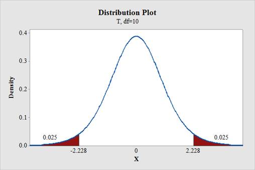
From the output, the critical point is, $t_{\frac{\alpha }{2}}=\pm 2.228$.

The confidence interval for ${\beta }_0$ is,

$\begin{array}{c}7.62327\pm 2.228\left(3.7556\right)=7.62327\pm \text{8}\text{.36748}\\ =\left(-\text{0}\text{.74421},\text{15}\text{.99075}\right)\end{array}$

Thus, the 95% confidence interval for ${\beta }_0$ is $\left(-\text{0}\text{.74421},\text{15}\text{.99075}\right)$.

Confidence interval for ${\beta }_1$:

The formula for confidence interval is, ${\widehat{\beta }}_1\pm t_{\frac{\alpha }{2}}{s}_{{\widehat{\beta }}_1}$.

The value of $s_{{\widehat{\beta }}_1}$ is calculated as follows:

$\begin{array}{c}{s}_{{\widehat{\beta }}_1}=\frac{s}{\sqrt{{\displaystyle \sum _{i=1}^n{\left(x_i-\overline{x}\right)}^2}}}\\ =\frac{4.24217}{\sqrt{6,032}}\\ =\frac{4.24217}{\text{77}\text{.66595}}\\ =\text{0}\text{.0546207}\end{array}$

The confidence interval for slope is,

$\begin{array}{c}0.329642\pm 2.228\left(0.0546207\right)=0.329642\pm \text{0}\text{.121695}\\ =\left(\text{0}\text{.207947},\text{0}\text{.451337}\right)\end{array}$

Thus, the 95% confidence interval for slope is $\left(\text{0}\text{.207947},\text{0}\text{.451337}\right)$.

To determine

Check whether the data provide sufficient evidence to conclude that the claim is false.

Answer to Problem 1E

The claim is false.

Explanation of Solution

Calculation:

Here, the claim is that the yield increases by more than 0.5 for each 1º C increase in temperature.

State the null and alternative hypotheses.

Null hypothesis:

$H_0:{\beta }_1\ge 0.5$

Alternative hypothesis:

$H_1:{\beta }_1<0.5$

Test statistic:

$\begin{array}{c}t=\frac{{\widehat{\beta }}_1-{\beta }_1}{s_{{\widehat{\beta }}_1}}\\ =\frac{0.329642-0.5}{0.0546207}\\ =\frac{-\text{0}\text{.170358}}{0.0546207}\\ =-3.12\end{array}$

Thus, the test statistic is –3.12.

P-value:

Software Procedure:

Step-by-step procedure to obtain the critical point using the MINITAB software:

• Choose Graph > Probability Distribution Plot choose View Probability > OK.
• From Distribution, choose ‘t’ distribution.
• In Degrees of freedom, enter 10.
• Click the Shaded Area tab.
• Choose X Value and Left Tail for the region of the curve to shade.
• Enter the data value as –3.12.
• Click OK.

Output using the MINITAB software is given below:

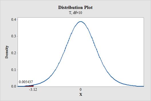
Thus, the P-value is 0.0054.

Conclusion:

Here, the P-value is small.

That is, the P-value is less than the level of significance, 0.05.

Therefore, the null hypothesis is rejected.

Hence, the given claim is false.

To determine

Find the 95% confidence interval for the mean yield at a temperature of 40º C.

Answer to Problem 1E

The 95% confidence interval for the mean yield at a temperature of 40º C is $\left(\text{16}\text{.72235},\text{24}\text{.89555}\right)$.

Explanation of Solution

Calculation:

The formula for confidence interval is, $\widehat{y}\pm t_{\frac{\alpha }{2}}{s}_{\widehat{y}}$.

Consider $x=40$. Therefore, the value of $\widehat{y}$ is,

$\begin{array}{c}\widehat{y}=\text{7}\text{.62327}+0.\text{329642}\left(40\right)\\ =\text{7}\text{.62327}+\text{13}\text{.18568}\\ =\text{20}\text{.80895}\end{array}$

The value of $s_{\widehat{y}}$ is calculated as follows:

$\begin{array}{c}{s}_{\widehat{y}}=s\sqrt{\frac{1}{n}+\frac{{\left(x-\overline{x}\right)}^2}{{\displaystyle \sum _{i=1}^n{\left(x_i-\overline{x}\right)}^2}}}\\ =4.242170\sqrt{\frac{1}{12}+\frac{{\left(40-65\right)}^2}{6,032}}\\ =4.242170\sqrt{\text{0}\text{.08333}+\text{0}\text{.103614}}\\ =\text{1}\text{.8342}\end{array}$

The 95% confidence interval for the mean yield at a temperature of 40º C is,

$\begin{array}{c}20.80895\pm 2.228\left(1.8342\right)=20.80895\pm \text{4}\text{.08660}\\ =\left(\text{16}\text{.72235},\text{24}\text{.89555}\right)\end{array}$

Thus, the 95% confidence interval for the mean yield at a temperature of 40º C is $\left(\text{16}\text{.72235},\text{24}\text{.89555}\right)$.

To determine

Find the 95% prediction interval for the yield of a particular reaction at a temperature of 40º C.

Answer to Problem 1E

The 95% prediction interval for the yield of a particular reaction at a temperature of 40º C is,

$\left(\text{10}\text{.51176},\text{31}\text{.10614}\right)$.

Explanation of Solution

Calculation:

The confidence interval formula is, $\widehat{y}\pm t_{\frac{\alpha }{2}}{s}_{\text{Pred}}$.

Consider $x=40$. Therefore, the value of $\widehat{y}$ is,

$\begin{array}{c}\widehat{y}=\text{7}\text{.62327}+0.\text{329642}\left(40\right)\\ =\text{7}\text{.62327}+\text{13}\text{.18568}\\ =\text{20}\text{.80895}\end{array}$

The value of $s_{\text{Pred}}$ is calculated as follows:

$\begin{array}{c}{s}_{\text{Pred}}=s\sqrt{1+\frac{1}{n}+\frac{{\left(x-\overline{x}\right)}^2}{{\displaystyle \sum _{i=1}^n{\left(x_i-\overline{x}\right)}^2}}}\\ =4.242170\sqrt{1+\frac{1}{12}+\frac{{\left(40-65\right)}^2}{6,032}}\\ =4.242170\sqrt{\text{1+0}\text{.08333}+\text{0}\text{.103614}}\\ =\text{4}\text{.62172}\end{array}$

The 95% prediction interval for the yield of a particular reaction at a temperature of 40º C is,

$\begin{array}{c}20.80895\pm 2.228\left(4.62172\right)=20.80895\pm \text{10}\text{.29719}\\ =\left(\text{10}\text{.51176},\text{31}\text{.10614}\right)\end{array}$

Thus, the 95% prediction interval for the yield of a particular reaction at a temperature of 40º C is,

$\left(\text{10}\text{.51176},\text{31}\text{.10614}\right)$.