Videos
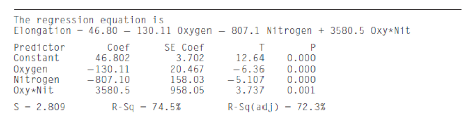
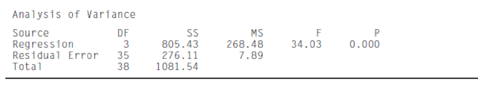
The article “Advances in Oxygen Equivalence liquations for Predicting the Properties of Titanium Welds” (D. Harwig, W. Ittiwattana, and H. Castner, The Welding Journal, 2001:126s–136s) reports an experiment to predict various properties of titanium welds. Among other properties, the elongation (in %) was measured, along with the oxygen content and nitrogen content (both in percent). The following MINITAB output presents results of fitting the model
- a. Predict the elongation for a weld with an oxygen content of 0.15% and a nitrogen content of 0.01%.
- b. If two welds both have a nitrogen content of 0.006%, and their oxygen content differs by 0.05%, what would you predict their difference in elongation to be?
- c. Two welds have identical oxygen contents, and nitrogen contents that differ by 0.005%. Is this enough information to predict their difference in elongation? If so, predict the elongation. If not, explain what additional information is needed.
a.
Find the predicted elongation percent of a weld with 0.15% of oxygen content and 0.01% of nitrogen content.
Answer to Problem 1SE
The predicted elongation percent of a weld with 0.15% of oxygen content and 0.01% of nitrogen content is likely to be 24.6%.
Explanation of Solution
Calculation:
The data represents the MINITAB output of the regression model
Multiple linear regression model:
A multiple linear regression model is given as
The ‘Coefficient’ column of the regression analysis MINITAB output gives the slopes corresponding to the respective variables stored in the column ‘Predictor’.
Let
From the accompanying MINITAB output, the intercept is
The estimates of the slopes are:
Thus, using the definition of a multiple regression model, the multiple regression equation is:
Here,
Predicted elongation percent of a weld:
Thus, the predicted elongation percent of a weld with 0.15% of oxygen content and 0.01% of nitrogen content is likely to be 24.6%.
b.
Find the change between the elongation percent of the two welds when the nitrogen content is 0.006% for both the welds with one weld containing 0.05% more oxygen content.
Answer to Problem 1SE
The elongation percent of two welds differ by –5.43% when the nitrogen content is 0.006% for both the welds with one weld containing 0.05% more oxygen content.
Explanation of Solution
Justification:
Slope in a multiple regression equation:
The slope
The multiple regression line is,
The coefficient or slope of Oxygen content in the regression model is
From this it can be said that, the value of elongation percent decreases by 130.11 for a 1% increase in Oxygen content, provided the effects of Nitrogen content is accounted for.
Here, both the welds have same Nitrogen content 0.006% and one weld has 0.05% more oxygen content than the other.
The change between the elongation percent of two welds is,
Thus, the elongation percent of two welds differ by –5.43% when the nitrogen content is 0.006% for both the welds with one weld containing 0.05% more oxygen content.
c.
Check whether it is possible to estimate the change in the elongation percent of the two welds when the nitrogen content is same for both the welds with one weld containing 0.005% more oxygen content.
If possible, predict the change.
Answer to Problem 1SE
No, it is not possible to estimate the change in the elongation percent of the two welds when the nitrogen content is same for both the welds with one weld containing 0.005% more oxygen content.
Explanation of Solution
Justification:
Slope in a multiple regression equation:
The slope
The multiple regression line is,
Here, the elongation is dependent on the nitrogen content, oxygen content and the interaction of nitrogen and oxygen content.
Hence, the coefficient of
Therefore, it is not possible to determine the change in the elongation percent only with the value of oxygen content.
Thus, it is not possible to estimate the change in the elongation percent of the two welds when the nitrogen content is same for both the welds with one weld containing 0.005% more oxygen content.
Want to see more full solutions like this?
Chapter 8 Solutions
Statistics for Engineers and Scientists - With Access
Additional Math Textbook Solutions
Introductory Statistics
An Introduction to Mathematical Statistics and Its Applications (6th Edition)
Elementary Statistics: A Step By Step Approach
Stats: Modeling the World Nasta Edition Grades 9-12
EBK STATISTICAL TECHNIQUES IN BUSINESS


- An agent for a property management company would like to be able to predict the monthly rental cost for apartments based on the size of the apartment as defined by square footage. A sample of the rent of 25 apartments in a college rental neighborhood was selected, and the information collected revealed the following: Apartment Size (Sq. Ft.) Monthly Rent ($) 1 850 950 2 1,450 1,600 3 1,085 1,200 4 1,232 1,500 5 718 950 6 1,485 1,700 7 1,136 1,650 8 726 935 9 700 875 10 956 1,150 11 1,100 1,400 12 1,285 1,650 13 1,985 2,300 14 1,369 1,800 15 1,175 1,400 16 1,225 1,450 17 1,245 1,100 18 1,259 1,700 19 1,150 1,200 20 896 1,150 21 1,361 1,600 22 1,040 1,650 23 755 1,200 24 1,000 800 25 1,200 1,750 e) Determine the coefficient of determination r2 and then completely interpret…arrow_forwardAn agent for a property management company would like to be able to predict the monthly rental cost for apartments based on the size of the apartment as defined by square footage. A sample of the rent of 25 apartments in a college rental neighborhood was selected, and the information collected revealed the following: Apartment Size (Sq. Ft.) Monthly Rent ($) 1 850 950 2 1,450 1,600 3 1,085 1,200 4 1,232 1,500 5 718 950 6 1,485 1,700 7 1,136 1,650 8 726 935 9 700 875 10 956 1,150 11 1,100 1,400 12 1,285 1,650 13 1,985 2,300 14 1,369 1,800 15 1,175 1,400 16 1,225 1,450 17 1,245 1,100 18 1,259 1,700 19 1,150 1,200 20 896 1,150 21 1,361 1,600 22 1,040 1,650 23 755 1,200 24 1,000 800 25 1,200 1,750 i) Determine a 95% interval estimate for the average rent of apartments with 1000…arrow_forwardThe attached data contains Part Quality data of three suppliers. At = 0.05, does Part Quality depend on Supplier, or should the cheapest Supplier be chosen?arrow_forward
- The article “Effect of Varying Solids Concentration and Organic Loading on the Performance of Temperature Phased Anaerobic Digestion Process” (S. Vandenburgh and T. Ellis, Water Environment Research, 2002:142–148) discusses experiments to determine the effect of the solids concentration on the performance of treatment methods for wastewater sludge. In the first experiment, the concentration of solids (in g/L) was 43.94 ± 1.18. In the second experiment, which was independent of the first, the concentration was 48.66 ± 1.76. Estimate the difference in the concentration between the two experiments, and find the uncertainty in the estimate.arrow_forwardThe spike stature of the plants grown from the seeds of the porcine separates (Dactylis glomerata L) collected from the University campus and İbradı Eynif pasture are given below. In this plant, compare whether there is a difference between regions in terms of spike height. Virgo Height (cm) Data obtained from plants collected from university campus 5 6 8 7 8 6 5 5 4 6 6 Data obtained from plants collected from Eynif pasture 12 9 11 9 9 11 9 10 11 10 Note: Your results interpretation according to two different possibilities (Do it separately, assuming that it is 0.07 and 0.04).arrow_forwardIn forestry, the diameter of a tree at breast height is used to model the height of the tree. Silviculturists working in British Columbia’s boreal forest conducted a series of spacing trials to predict the heights of several species of trees. The data are the breast height diameters (in centimeters) and heights (in meters) for a sample of 18 white spruce trees. B1 B2 18.9 20.0 15.5 16.8 19.4 20.2 20.0 20.0 29.8 20.2 19.8 18.0 20.3 17.8 20.0 19.2 22.0 22.3 16.6 18.8 15.5 16.9 13.7 16.3 27.5 21.4 20.3 19.2 22.9 19.8 14.1 18.5 10.1 12.1 5.8 8.0 B1: Breast Height Diameter of White spruce (cm) B2: Height (m) a) Plot the relationship using scatter diagram between the breast height diameters and the trees’ height. Are the breast height diameters and the trees’ height linearly related? What can you infer about the relationship between the two variables? Is a linear model appropriate? b) Compare the scatter plot in (a) with the correlation coefficient…arrow_forward
- Consider a cohort study to compare the mortality rate of myocardial infarction (MI) in men with sedentary work (exposed group) to men with physically active work (unexposed). If in the exposed, there were 36,000 person (man) years of observation and 126 deaths whereas the unexposed had 24,000 man-years of observation and 44 deaths. Compute the following a) Mortality rate in each cohort? b) What is the relative risk of dying, comparing these 2 groups? c) What is the attributable risk of sedentary work? d) What is the attributable benefit of physical activity? e) If we assume that MI is associated with the mortality in this cohort (causality), what proportion of the disease in the higher group is potentially preventable?arrow_forwardBased on data collected by the U.S. General Social Survey, a researcher examines the frequency with which adults responded to two questions. The first asked people if they resided in the same city or town now as when they were 16 years old (Residence). The second asked if they found life generally exciting, routine, or dull (Life). Using data from 2,791 people, the results are below. Life is Generally: Living in: Exciting Routine Dull Marginal n Same City or Town O = 489 E = O = 601 E = O = 64 E = 1154 Different Area O = 797 E = O = 763 E = O = 77 E = 1637 Marginal n 1286 1364 141 2791 Using the chi-square (χ2) test for independence, examine if the feelings people have about life in general are related to living in the same city or town as when a teen. State the hypotheses (H0 and H1). Find the critical value for α = .05, 1-tailed. Calculate the test statistic (χ2), filling in relevant portions of the…arrow_forwardIn a study attempting to replicate findings by Stephens, Atkins, & Kingston (2009), each participant was asked to plunge a hand into the icy water and keep it there as long as the pain would allow. In one condition, the participants repeated their favorite curse words while their hands were in the water. In the other condition, they repeated neutral words. The original research showed that, in addition to lowering the participants’ perception of pain, swearing also increased the amount of time they were able to tolerate the pain. Data similar to the results obtained in the study are shown in the following table: _____________Amount of Time (in Seconds)_ Participant Swear Words Neutral Words 1 94 59 2 70 61 3 52 47 4…arrow_forward
- In a study attempting to replicate findings by Stephens, Atkins, & Kingston (2009), each participant was asked to plunge a hand into the icy water and keep it there as long as the pain would allow. In one condition, the participants repeated their favorite curse words while their hands were in the water. In the other condition, they repeated neutral words. The original research showed that, in addition to lowering the participants’ perception of pain, swearing also increased the amount of time they were able to tolerate the pain. Data similar to the results obtained in the study are shown in the following table: _____________Amount of Time (in Seconds)_ Participant Swear Words Neutral Words 1 94 59 2 70 61 3 52 47 4…arrow_forwardIn a summary report given by Ing. Pobbi on the lengths of ironrods produced by two machines, he stated that the variability ofmachine A was higher compared to that of machine B. Critiquethe report of the Engineer given data on the length of rodsproduced given as; MachineA(cm): 380 410 280 310 305 360 270 355 400 Machine B(m): 1.1 1.3 1.2 2.0 1.5 1.6 1.4 1.6 1.7arrow_forwardrofessor Cornish studied rainfall cycles and sunspot cycles. (Reference: Australian Journal of Physics, Vol. 7, pp. 334-346.) Part of the data include amount of rain (in mm) for 6-day intervals. The following data give rain amounts for consecutive 6-day intervals at Adelaide, South Australia. 7 28 7 1 69 3 1 4 22 7 16 4 54 160 60 73 27 3 3 1 7 144 107 4 91 44 1 8 4 22 4 59 116 52 4 155 42 24 11 43 3 24 19 74 26 63 110 39 34 71 52 39 8 0 15 2 14 9 1 2 4 9 6 10 (i) Find the median. (Use 1 decimal place.)(ii) Convert this sequence of numbers to a sequence of symbols A and B, where A indicates a value above the median and B a value below the median. Test the sequence for randomness about the median at the 5% level of significance. (b) Find the number of runs R, n1, and n2. Let n1 = number of values above the median and n2 = number of values below the median. R n1 n2 (c) In the case, n1 > 20, we cannot use Table 10 of Appendix II to find the critical…arrow_forward
 Glencoe Algebra 1, Student Edition, 9780079039897...AlgebraISBN:9780079039897Author:CarterPublisher:McGraw Hill