Chapter 8, Problem 23SE

The article “Estimating Resource Requirements at Conceptual Design Stage Using Neural Networks” (A. Elazouni, I. Nosair, et al., Journal of Computing in Civil Engineering, 1997:217–223) suggests that certain resource requirements in the construction of concrete silos can be predicted from a model. These include the quantity of concrete in m³ (y), the number of crew-days of labor (z), or the number of concrete mixer hours (w) needed for a particular job. Table SE23A defines 23 potential independent variables that can be used to predict y, z, or w. Values of the dependent and independent variables, collected on 28 construction jobs, are presented in Table SE23B (page 659) and Table SE23C (page 660). Unless otherwise stated, lengths are in meters, areas in metres, and volumes in m³

1. a. Using best subsets regression, find the model that is best for predicting y according to the adjusted R² criterion.
2. b. Using best subsets regression, find the model that is best for predicting y according to the minimum Mallows C_p criterion.
3. c. Find a model for predicting y using stepwise regression. Explain the criterion you are using to determine which variables to add to or drop from the model.
4. d. Using best subsets regression, find the model that is best for predicting z according to the adjusted R² criterion.
5. e. Using best subsets regression, find the model that is best for predicting z according to the minimum Mallows C_p criterion.
6. f. Find a model for predicting z using stepwise regression. Explain the criterion you are using to determine which variables to add to or drop from the model.
7. g. Using best subsets regression, find the model that is best for predicting w according to the adjusted R criterion.
8. h. Using best subsets regression, find the model that is best for predicting w according to the minimum Mallows C_p criterion.
9. i. Find a model for predicting w using stepwise regression. Explain the criterion you are using to determine which variables to add to or drop from the model.

TABLE SF23A Descriptions of Variables for Exercise 73

x1	Number of bins	x13	Breadth-to-thickness ratio
x2	Maximum required concrete per hour	x14	Perimeter of complex
x3	Height	x15	Mixer capacity
x4	Sliding rate of the slipform (m/day)	x16	Density of stored material
x5	Number of construction stages	x17	Waste percent in reinforcing steel
x6	Perimeter of slipform	x18	Waste percent in concrete
x7	Volume of silo complex	x19	Number of workers in concrete crew
x8	Surface area of silo walls	x20	Wall thickness (cm)
x9	Volume of one bin	x21	Number of reinforcing steel crew s
x10	Wall-to-floor areas	x22	Number of workers in forms crew
x11 x12	Number of lifting jacks Length-to-thickness ratio	x23	Length-to-breadth ratio

To determine

Find the best regression model to predict the dependent variable y using the adjusted-$R^2$ criterion.

Answer to Problem 23SE

The best regression model to predict the dependent variable y using the adjusted-$R^2$ criterion is $\underset{\_}{\widehat{y}=\left(\begin{array}{l}-1,570-24.91x_1+196.9x_2+8.87x_3-2.236x_6-0.0776x_7+0.05733x_8\\ -1.306x_9-12.23x_{11}+44.1x_{13}+4.188x_{14}+0.971x_{16}+74.8x_{18}+21.7x_{19}\\ -18.25x_{20}+82.6x_{21}-37.6x_{22}+330x_{23}\end{array}\right)}$.

Explanation of Solution

Calculation:

The data represents the values of 23 potential independent variables that are used to predict three dependent variables quantity of concrete in ${\text{m}}^{\text{3}}$$\left(y\right)$, the number of crew-days of labor $\left(z\right)$ and number of concrete mixture hours $\left(w\right)$. The data is collected on 28 construction jobs.

Multiple linear regression model:

A multiple linear regression model is given as $y_i={\beta }_0+{\beta }_1{x}_{1i}+\mathrm{...}+{\beta }_k{x}_{ki}+{\epsilon }_i$ where $y_i$ is the response variable, and $x_{1i},x_{2i},\mathrm{...},x_{ki}$ are the k predictor variables. The quantities ${\beta }_0,{\beta }_1,\mathrm{...},{\beta }_k$ are the slopes corresponding to $x_{1i},x_{2i},\mathrm{...},x_{ki}$ respectively.${\widehat{\beta }}_0$ is the estimated intercept of the line, from the sample data.

Let $x_1,x_2,\mathrm{...},x_{23}$ be the independent variables and $y_1,y_2,y_3$ be the dependent variables.

Adjusted $R^2$or$R_a^2$:

An important utility of the adjusted coefficient of multiple determination or $R_a^2$ is to find the best subset of the predictors, that can predict the response variable. The best subset may be a smaller subset of all the predictors and need not necessarily be a larger subset, as long as it predicts the response variable accurately. The subset with larger $R_a^2$ is considered to be best subset for prediction.

The adjusted coefficient of multiple determination, $R_a^2$, is given by:

$R_a^2=1-\frac{\frac{SSE}{n-\left(k+1\right)}}{\frac{SST}{n-1}}$.

Subset regression:

Software procedure:

Step by step procedure to obtain regression using MINITAB software is given as,

• Choose Stat > Regression > Regression> Best subsets.
• In Response, enter the numeric column containing the response data Y.
• In Model, enter the numeric column containing the predictor variablesX1, X2,…,X23.
• Click OK.

Output obtained from MINITAB is given below:

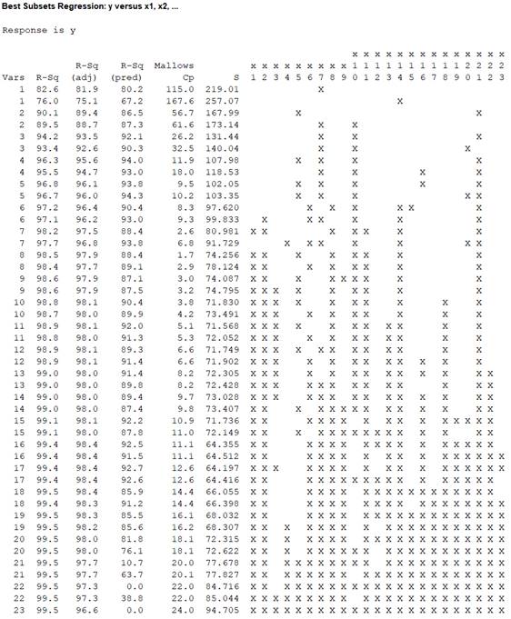
With increasing subset size, the value of $R^2$ always increases or remains constant, but never decreases. On the other hand, the value of $R_a^2$ may increase or decrease with increasing subset size, depending upon whether the subset is better or worse for prediction purposes.

From the obtained MINITAB output, it is clear that the highest value of adjusted $R^2$ is 98.4 corresponding to two 16 predictor variable models, two 17 predictor variable models and one 18 predictor variable model.

From these 5 models, the best model might be anyone of the three. Also, best subset model suggests that many other models will be equally likely good.

By observing these 5 models, it is clear that the highest predicted $R^2$ is 92.7, corresponding to the model with variables, $x_1,x_2,x_3,x_6,x_7,x_8,x_9,x_{11},x_{13},x_{14},x_{16},x_{18},x_{19},x_{20},x_{21},x_{22}\text{and }{x}_{23}$.

The value of adjusted $R_a^2$ is the highest for predictors $x_1,x_2,x_3,x_6,x_7,x_8,x_9,x_{11},x_{13},x_{14},x_{16},x_{18},x_{19},x_{20},x_{21},x_{22}\text{and }{x}_{23}$. However, the subset with highest value of adjusted $R_a^2$ is considered to be best subset for prediction.

Thus, provided other factors do not affect the analysis it could be most preferable to use the regression equation corresponding to the predictors, $x_1,x_2,x_3,x_6,x_7,x_8,x_9,x_{11},x_{13},x_{14},x_{16},x_{18},x_{19},x_{20},x_{21},x_{22}\text{and }{x}_{23}$.

Hence, the variables for the model using the adjusted-$R^2$ criterion is $x_1,x_2,x_3,x_6,x_7,x_8,x_9,x_{11},x_{13},x_{14},x_{16},x_{18},x_{19},x_{20},x_{21},x_{22}\text{and }{x}_{23}$.

Regression:

Software procedure:

Step by step procedure to obtain regression using MINITAB software is given as,

• Choose Stat > Regression > General Regression.
• In Response, enter the numeric column containing the response dataY.
• In Model, enter the numeric column containing the predictor variables X1,X2,X3,X6,X7,X8,X9,X11,X13,X14,X16,X18,X19,X20, x21, X22 and X23.
• Click OK.

Output obtained from MINITAB is given below:

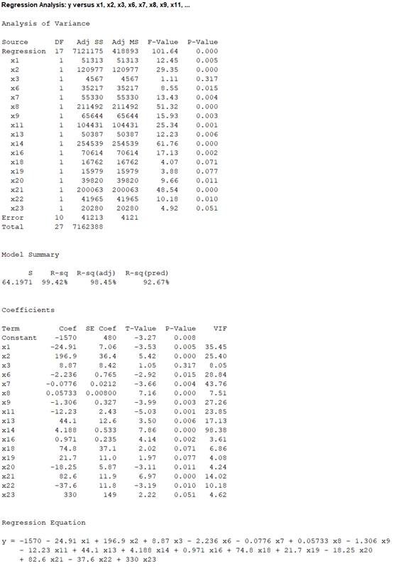
The ‘Coefficient’ column of the regression analysis MINITAB output gives the slopes corresponding to the respective variables stored in the column ‘Term’.

A careful inspection of the output shows that the fitted model is:

$\widehat{y}=\left(\begin{array}{l}-1,570-24.91x_1+196.9x_2+8.87x_3-2.236x_6-0.0776x_7+0.05733x_8\\ -1.306x_9-12.23x_{11}+44.1x_{13}+4.188x_{14}+0.971x_{16}+74.8x_{18}+21.7x_{19}\\ -18.25x_{20}+82.6x_{21}-37.6x_{22}+330x_{23}\end{array}\right)$.

Hence, the best multiple linear regression model using adjusted-$R^2$ criterion for the given data is:

$\underset{\_}{\widehat{y}=\left(\begin{array}{l}-1,570-24.91x_1+196.9x_2+8.87x_3-2.236x_6-0.0776x_7+0.05733x_8\\ -1.306x_9-12.23x_{11}+44.1x_{13}+4.188x_{14}+0.971x_{16}+74.8x_{18}+21.7x_{19}\\ -18.25x_{20}+82.6x_{21}-37.6x_{22}+330x_{23}\end{array}\right)}$.

To determine

Find the best regression model to predict the dependent variable y using the Mallows’ $C_p$ criterion.

Answer to Problem 23SE

The best regression model to predict the dependent variable y using the Mallows’ $C_p$ criterion is $\underset{\_}{\widehat{y}=\left(\begin{array}{l}-666-24.78x_1+76.5x_2+122x_5+0.02425x_8\\ +20.4x_{10}-7.13x_{11}+2.447x_{14}+47.85x_{21}\end{array}\right)}$.

Explanation of Solution

Mallows’ $C_p$:

An important utility of the Mallows’ $C_p$ criterion is to compare between regression equations of subsets having different sizes, all taken from the same all-subsets regression.

Mallows’ $C_p$ criterion is given as:

$C_p=\frac{SS{E}_{subset}}{MS{E}_{all}}-\left(n-2p\right)$, where $SS{E}_{subset}$ denotes the error sum of squares of the current model and $MS{E}_{all}$ denotes the error mean square for the set of all potential predictors, n is the sample size and $p=k+1$, with k being the number of predictors.

The predictor with the lowest value of $C_p$ or the value of $C_p$ closest to p is chosen to predict the response variable.

From the obtained MINITAB output, it is clear that the lowest value of a Mallows’ $C_p$ is 1.7 corresponding to 8 predictor variable model.

The value of $C_p$ is the lowest for predictors $x_1,x_2,x_5,x_8,x_{10},x_{11},x_{14}\text{and }{x}_{21}$. However, the subset with lowest value of $C_p$ is considered to be best subset for prediction.

Thus, depending upon the factors affecting the analysis it would be most preferable to use the regression equation corresponding to the predictors $x_1,x_2,x_5,x_8,x_{10},x_{11},x_{14}\text{and }{x}_{21}$.

Hence, the variables for the model using the Mallows’ $C_p$ criterion are $x_1,x_2,x_5,x_8,x_{10},x_{11},x_{14}\text{and }{x}_{21}$.

Regression:

Software procedure:

Step by step procedure to obtain regression using MINITAB software is given as,

• Choose Stat > Regression > General Regression.
• In Response, enter the numeric column containing the response dataY.
• In Model, enter the numeric column containing the predictor variablesX1, X2, X5, X8, X10, X11, X14 and X21.
• Click OK.

Output obtained from MINITAB is given below:

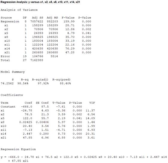
The ‘Coefficient’ column of the regression analysis MINITAB output gives the slopes corresponding to the respective variables stored in the column ‘Term’.

A careful inspection of the output shows that the fitted model is:

$\widehat{y}=\left(\begin{array}{l}-666-24.78x_1+76.5x_2+122x_5+0.02425x_8\\ +20.4x_{10}-7.13x_{11}+2.447x_{14}+47.85x_{21}\end{array}\right)$.

Hence, the best multiple linear regression model using Mallows’ $C_p$ criterion for the given data is:

$\underset{\_}{\widehat{y}=\left(\begin{array}{l}-666-24.78x_1+76.5x_2+122x_5+0.02425x_8\\ +20.4x_{10}-7.13x_{11}+2.447x_{14}+47.85x_{21}\end{array}\right)}$.

To determine

Obtain regression equation to predict y using the stepwise regression method.

Answer to Problem 23SE

The regression equation to predict y using the stepwise regression method is $\underset{\_}{\widehat{y}=-928+142.4x_5+0.0817x_7+21.7x_{10}+0.413x_{16}+45.67x_{21}}$

Explanation of Solution

Stepwise regression:

The stepwise regression method to develop a regression model is a combination of the forward selection and backward elimination methods. The method starts with no predictors and then including or eliminating at most one predictor at each step, such that the predictors satisfy the conditions:

• The forward selection method is used to add a predictor with the largest value of t-statistic among all predictors that are not currently in the model, such that the absolute value of this largest t-statistic must be greater than a pre-specified value, $t_{enter}$.
• The backward elimination method is applied to the model with at least one predictor, to remove the predictor from the model, which has the smallest t-statistic value and less than a pre-specified value, $t_{remove}$. The removed variables can be considered in future steps for inclusion.

Since, the values for ${\alpha }_{enter}$ and ${\alpha }_{remove}$ are not specified. The prior values ${\alpha }_{enter}={\alpha }_{remove}=0.15$ can be used.

Regression:

Software procedure:

Step by step procedure to obtain regression using MINITAB software is given as,

• Choose Stat > Regression > General Regression.
• In Response, enter the numeric column containing the response dataY.
• In Model, enter the numeric column containing the predictor variables X1,X2,…,X23.
• In Stepwise, select method as Stepwise.
• Enter 0.15 in Alpha to enter and 0.15 as Alpha to remove.
• Click OK.

Output obtained from MINITAB is given below:

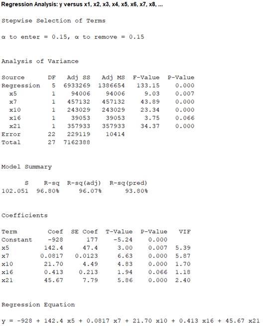
The ‘Coefficient’ column of the regression analysis MINITAB output gives the slopes corresponding to the respective variables stored in the column ‘Term’.

A careful inspection of the output shows that the fitted model is:

$\widehat{y}=-928+142.4x_5+0.0817x_7+21.7x_{10}+0.413x_{16}+45.67x_{21}$.

Hence, the regression equation to predict y using the stepwise regression method is:

$\underset{\_}{\widehat{y}=-928+142.4x_5+0.0817x_7+21.7x_{10}+0.413x_{16}+45.67x_{21}}$.

To determine

Find the best regression model to predict the dependent variable z using the adjusted-$R^2$ criterion.

Answer to Problem 23SE

The best regression model to predict the dependent variable z using the adjusted-$R^2$ criterion is $\underset{\_}{\widehat{z}=\left(\begin{array}{l}-8,663-313.3x_3-14.46x_6+0.358x_7-0.0787x_8\\ +14x_9+230.2x_{10}-188.2x_{13}+5.41x_{14}+1,928x_{15}-8.25x_{16}+294.9x_{19}\\ +129.8x_{22}-3,021x_{23}\end{array}\right)}$.

Explanation of Solution

Calculation:

Subset regression:

Software procedure:

Step by step procedure to obtain regression using MINITAB software is given as,

• Choose Stat > Regression > Regression> Best subsets.
• In Response, enter the numeric column containing the response data Z.
• In Model, enter the numeric column containing the predictor variablesX1, X2,…,X23.
• Click OK.

Output obtained from MINITAB is given below:

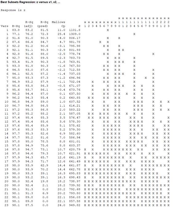
From the obtained MINITAB output, it is clear that the highest value of adjusted $R^2$ is 95.4 corresponding to two 12 predictor variable models and one 13 predictor variable model.

From these 3 models, the best model might be anyone of the three. Since, best subset model suggests that many other models will be equally likely good.

By observing these 5 models, it is clear that the highest predicted $R^2$ is 85.9, corresponding to the model with variables, $x_3,x_6,x_7,x_8,x_9,x_{10},x_{13},x_{14},x_{15},x_{16},x_{19},x_{22}\text{and }{x}_{23}$.

The value of adjusted $R_a^2$ is the highest for predictors $x_3,x_6,x_7,x_8,x_9,x_{10},x_{13},x_{14},x_{15},x_{16},x_{19},x_{22}\text{and }{x}_{23}$. However, the subset with highest value of adjusted $R_a^2$ is considered to be best subset for prediction.

Thus, provided other factors do not affect the analysis it could be most preferable to use the regression equation corresponding to the predictors, $x_3,x_6,x_7,x_8,x_9,x_{10},x_{13},x_{14},x_{15},x_{16},x_{19},x_{22}\text{and }{x}_{23}$.

Hence, the variables for the model using the adjusted-$R^2$ criterion is $x_3,x_6,x_7,x_8,x_9,x_{10},x_{13},x_{14},x_{15},x_{16},x_{19},x_{22}\text{and }{x}_{23}$.

Regression:

Software procedure:

Step by step procedure to obtain regression using MINITAB software is given as,

• Choose Stat > Regression > General Regression.
• In Response, enter the numeric column containing the response dataZ.
• In Model, enter the numeric column containing the predictor variables X3, X6, X7, X8, X9, X10, X13, X14, X15, X16, X19, X22 and X23.
• Click OK.

Output obtained from MINITAB is given below:

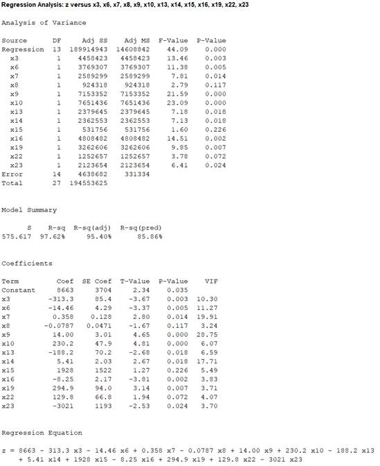
The ‘Coefficient’ column of the regression analysis MINITAB output gives the slopes corresponding to the respective variables stored in the column ‘Term’.

A careful inspection of the output shows that the fitted model is:

$\widehat{z}=\left(\begin{array}{l}-8,663-313.3x_3-14.46x_6+0.358x_7-0.0787x_8\\ +14x_9+230.2x_{10}-188.2x_{13}+5.41x_{14}+1,928x_{15}-8.25x_{16}+294.9x_{19}\\ +129.8x_{22}-3,021x_{23}\end{array}\right)$.

Hence, the best multiple linear regression modelto predict z using adjusted-$R^2$ criterion for the given data is:

$\underset{\_}{\widehat{z}=\left(\begin{array}{l}-8,663-313.3x_3-14.46x_6+0.358x_7-0.0787x_8\\ +14x_9+230.2x_{10}-188.2x_{13}+5.41x_{14}+1,928x_{15}-8.25x_{16}+294.9x_{19}\\ +129.8x_{22}-3,021x_{23}\end{array}\right)}$.

To determine

Find the best regression model to predict the dependent variable z using the Mallows’ $C_p$ criterion.

Answer to Problem 23SE

The best regression model to predict the dependent variable z using the Mallows’ $C_p$ criterion is $\underset{\_}{\widehat{z}=\left(-1,661+0.6715x_7+134.3x_{10}\right)}$.

Explanation of Solution

From the obtained MINITAB output, it is clear that the lowest value of a Mallows’ $C_p$ is –4.0 corresponding to 8 predictor variable model.

The value of $C_p$ is the lowest for predictors $x_7\text{and }{x}_{10}$. However, the subset with lowest value of $C_p$ is considered to be best subset for prediction.

Thus, depending upon the factors affecting the analysis it would be most preferable to use the regression equation corresponding to the predictors $x_7\text{and }{x}_{10}$.

Hence, the variables for the model using the Mallows’ $C_p$ criterion are $x_7\text{and }{x}_{10}$.

Regression:

Software procedure:

Step by step procedure to obtain regression using MINITAB software is given as,

• Choose Stat > Regression > General Regression.
• In Response, enter the numeric column containing the response dataZ.
• In Model, enter the numeric column containing the predictor variablesX1 and X10.
• Click OK.

Output obtained from MINITAB is given below:

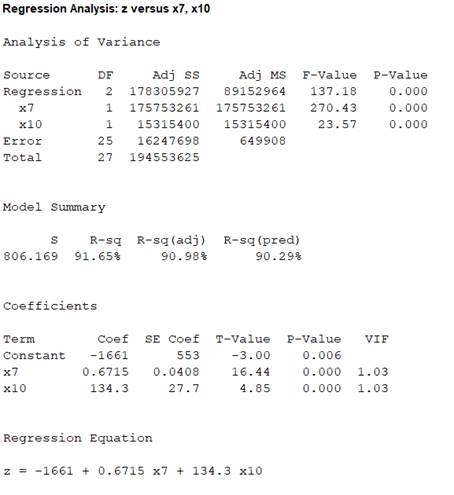
The ‘Coefficient’ column of the regression analysis MINITAB output gives the slopes corresponding to the respective variables stored in the column ‘Term’.

A careful inspection of the output shows that the fitted model is:

$\widehat{z}=\left(-1,661+0.6715x_7+134.3x_{10}\right)$.

Hence, the best multiple linear regression model using Mallows’ $C_p$ criterion for the given data is:

$\underset{\_}{\widehat{z}=\left(-1,661+0.6715x_7+134.3x_{10}\right)}$.

To determine

Obtain regression equation to predict z using the stepwise regression method.

Answer to Problem 23SE

The regression equation to predict z using the stepwise regression method is $\underset{\_}{\widehat{z}=-1,661+0.6715x_7+134.3x_{10}}$

Explanation of Solution

Stepwise regression:

The stepwise regression method to develop a regression model is a combination of the forward selection and backward elimination methods. The method starts with no predictors and then including or eliminating at most one predictor at each step, such that the predictors satisfy the conditions:

• The forward selection method is used to add a predictor with the largest value of t-statistic among all predictors that are not currently in the model, such that the absolute value of this largest t-statistic must be greater than a pre-specified value, $t_{enter}$.
• The backward elimination method is applied to the model with at least one predictor, to remove the predictor from the model, which has the smallest t-statistic value and less than a pre-specified value, $t_{remove}$. The removed variables can be considered in future steps for inclusion.

Since, the values for ${\alpha }_{enter}$ and ${\alpha }_{remove}$ are not specified. The prior values ${\alpha }_{enter}={\alpha }_{remove}=0.15$ can be used.

Regression:

Software procedure:

Step by step procedure to obtain regression using MINITAB software is given as,

• Choose Stat > Regression > General Regression.
• In Response, enter the numeric column containing the response data Z.
• In Model, enter the numeric column containing the predictor variables X1,X2,…,X23.
• In Stepwise, select method as Stepwise.
• Enter 0.15 in Alpha to enter and 0.15 as Alpha to remove.
• Click OK.

Output obtained from MINITAB is given below:

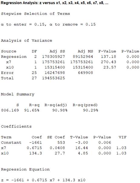
The ‘Coefficient’ column of the regression analysis MINITAB output gives the slopes corresponding to the respective variables stored in the column ‘Term’.

A careful inspection of the output shows that the fitted model is:

$\widehat{z}=-1,661+0.6715x_7+134.3x_{10}$.

Hence, the regression equation to predict z using the stepwise regression method is:

$\underset{\_}{\widehat{z}=-1,661+0.6715x_7+134.3x_{10}}$.

To determine

Find the best subset regression model to predict the dependent variable w using the adjusted-$R^2$ criterion.

Answer to Problem 23SE

The best regression model to predict the dependent variable w using the adjusted-$R^2$ criterion is $\underset{\_}{\widehat{w}=\left(\begin{array}{l}701-21.7x_2-20x_3+21.8x_4+62.6x_5+0.01616x_7-0.01269x_8\\ +1.132x_9+15.24x_{10}+1.110x_{11}-20.52x_{13}-90.2x_{15}-0.7744x_{16}\\ +7.56x_{19}+5.92x_{20}-7.55x_{21}+12.99x_{22}-271.3x_{23}\end{array}\right)}$.

Explanation of Solution

Calculation:

Subset regression:

Software procedure:

Step by step procedure to obtain regression using MINITAB software is given as,

• Choose Stat > Regression > Regression> Best subsets.
• In Response, enter the numeric column containing the response data W.
• In Model, enter the numeric column containing the predictor variablesX1, X2,…,X23.
• Click OK.

Output obtained from MINITAB is given below:

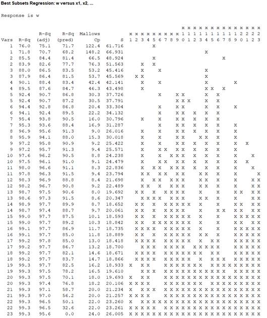
From the obtained MINITAB output, it is clear that the highest value of adjusted $R^2$ is 97.8 corresponding to 17 predictor variable model.

The value of adjusted $R_a^2$ is the highest for predictors $x_2,x_3,x_4,x_5,x_7,x_8,x_9,x_{10},x_{11},x_{13},x_{15},x_{16},x_{19},x_{20},x_{21},x_{22}\text{and }{x}_{23}$. However, the subset with highest value of adjusted $R_a^2$ is considered to be best subset for prediction.

Thus, provided other factors do not affect the analysis it could be most preferable to use the regression equation corresponding to the predictors, $x_2,x_3,x_4,x_5,x_7,x_8,x_9,x_{10},x_{11},x_{13},x_{15},x_{16},x_{19},x_{20},x_{21},x_{22}\text{and }{x}_{23}$.

Hence, the variables for the model using the adjusted-$R^2$ criterion is $x_2,x_3,x_4,x_5,x_7,x_8,x_9,x_{10},x_{11},x_{13},x_{15},x_{16},x_{19},x_{20},x_{21},x_{22}\text{and }{x}_{23}$.

Regression:

Software procedure:

Step by step procedure to obtain regression using MINITAB software is given as,

• Choose Stat > Regression > General Regression.
• In Response, enter the numeric column containing the response dataW.
• In Model, enter the numeric column containing the predictor variablesX2, X3,X4, X5, X7, X8, X9, X10, X11, X13, X15, X16, X19, X20, X21, X22 and X23.
• Click OK.

Output obtained from MINITAB is given below:

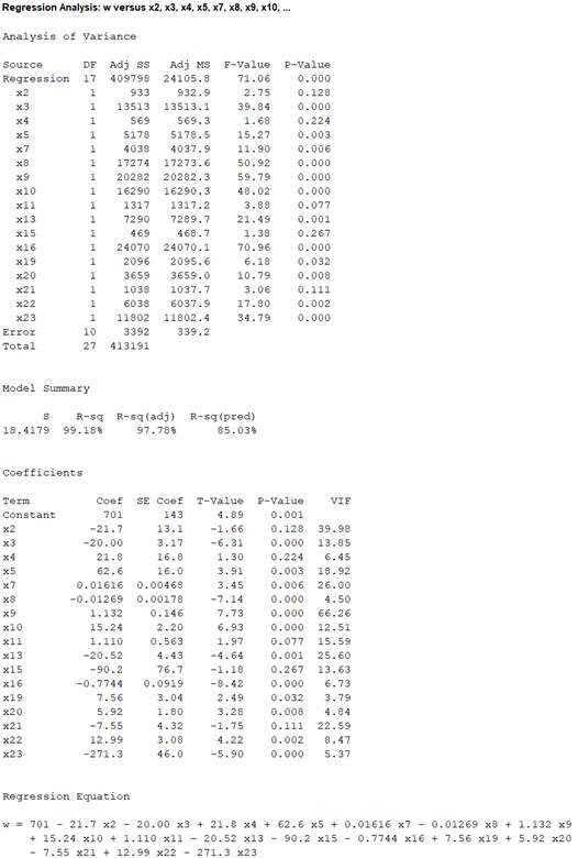
The ‘Coefficient’ column of the regression analysis MINITAB output gives the slopes corresponding to the respective variables stored in the column ‘Term’.

A careful inspection of the output shows that the fitted model is:

$\widehat{w}=\left(\begin{array}{l}701-21.7x_2-20x_3+21.8x_4+62.6x_5+0.01616x_7-0.01269x_8\\ +1.132x_9+15.24x_{10}+1.110x_{11}-20.52x_{13}-90.2x_{15}-0.7744x_{16}\\ +7.56x_{19}+5.92x_{20}-7.55x_{21}+12.99x_{22}-271.3x_{23}\end{array}\right)$.

Hence, the best multiple linear regression model to predict w using adjusted-$R^2$ criterion for the given data is:

$\underset{\_}{\widehat{w}=\left(\begin{array}{l}701-21.7x_2-20x_3+21.8x_4+62.6x_5+0.01616x_7-0.01269x_8\\ +1.132x_9+15.24x_{10}+1.110x_{11}-20.52x_{13}-90.2x_{15}-0.7744x_{16}\\ +7.56x_{19}+5.92x_{20}-7.55x_{21}+12.99x_{22}-271.3x_{23}\end{array}\right)}$.

To determine

Find the best regression model to predict the dependent variable w using the Mallows’ $C_p$ criterion.

Answer to Problem 23SE

The best regression model to predict the dependent variable w using the Mallows’ $C_p$ criterion is $\underset{\_}{\widehat{w}=\left(\begin{array}{l}567-23.58x_2-16.77x_3+90.48x_5+0.00823x_7-0.01100x_8\\ +0.896x_9+12.13x_{10}-11.98x_{13}-0.6730x_{16}\\ +11.10x_{19}+4.64x_{20}+11.11x_{22}-217.8x_{23}\end{array}\right)}$.

Explanation of Solution

From the obtained MINITAB output, it is clear that the lowest value of aMallows’ $C_p$ is 8.0 corresponding to 13 predictor variable model.

The value of $C_p$ is the lowest for predictors $x_2,x_3,x_5,x_7,x_8,x_9,x_{10},x_{13},x_{16},x_{19},x_{20},x_{22}\text{and }{x}_{23}$. However, the subset with lowest value of $C_p$ is considered to be best subset for prediction.

Thus, depending upon the factors affecting the analysis it would be most preferable to use the regression equation corresponding to the predictors $x_2,x_3,x_5,x_7,x_8,x_9,x_{10},x_{13},x_{16},x_{19},x_{20},x_{22}\text{and }{x}_{23}$.

Hence, the variables for the model using the Mallows’ $C_p$ criterion are $x_2,x_3,x_5,x_7,x_8,x_9,x_{10},x_{13},x_{16},x_{19},x_{20},x_{22}\text{and }{x}_{23}$.

Regression:

Software procedure:

Step by step procedure to obtain regression using MINITAB software is given as,

• Choose Stat > Regression > General Regression.
• In Response, enter the numeric column containing the response dataW.
• In Model, enter the numeric column containing the predictor variablesX2, X3, X5, X7, X8, X9, X10, X13, X16, X19, X20, X22 and X23.
• Click OK.

Output obtained from MINITAB is given below:

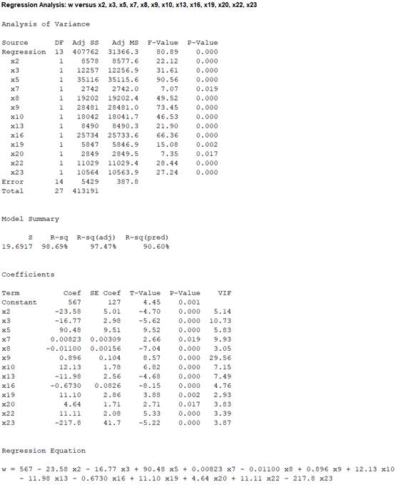
The ‘Coefficient’ column of the regression analysis MINITAB output gives the slopes corresponding to the respective variables stored in the column ‘Term’.

A careful inspection of the output shows that the fitted model is:

$\widehat{w}=\left(\begin{array}{l}567-23.58x_2-16.77x_3+90.48x_5+0.00823x_7-0.01100x_8\\ +0.896x_9+12.13x_{10}-11.98x_{13}-0.6730x_{16}\\ +11.10x_{19}+4.64x_{20}+11.11x_{22}-217.8x_{23}\end{array}\right)$.

Hence, the best multiple linear regression model using Mallows’ $C_p$ criterion for the given data is:

$\underset{\_}{\widehat{w}=\left(\begin{array}{l}567-23.58x_2-16.77x_3+90.48x_5+0.00823x_7-0.01100x_8\\ +0.896x_9+12.13x_{10}-11.98x_{13}-0.6730x_{16}\\ +11.10x_{19}+4.64x_{20}+11.11x_{22}-217.8x_{23}\end{array}\right)}$.

To determine

Obtain regression equation to predict w using the stepwise regression method.

Explain the criterion that is using to determine which variable to add to or drop from the model.

Answer to Problem 23SE

The regression equation to predict w using the stepwise regression method is $\underset{\_}{\widehat{w}=\left(\begin{array}{l}130.9-28.08x_2+113.49x_5+0.1680x_9-0.2022x_{16}\\ +11.42x_{19}+12.07x_{21}-78.4x_{23}\end{array}\right)}$

Explanation of Solution

Stepwise regression:

The stepwise regression method to develop a regression model is a combination of the forward selection and backward elimination methods. The method starts with no predictors and then including or eliminating at most one predictor at each step, such that the predictors satisfy the conditions:

• The forward selection method is used to add a predictor with the largest value of t-statistic among all predictors that are not currently in the model, such that the absolute value of this largest t-statistic must be greater than a pre-specified value, $t_{enter}$.
• The backward elimination method is applied to the model with at least one predictor, to remove the predictor from the model, which has the smallest t-statistic value and less than a pre-specified value, $t_{remove}$. The removed variables can be considered in future steps for inclusion.

Since, the values for ${\alpha }_{enter}$ and ${\alpha }_{remove}$ are not specified. The prior values ${\alpha }_{enter}={\alpha }_{remove}=0.15$ can be used.

Regression:

Software procedure:

Step by step procedure to obtain regression using MINITAB software is given as,

• Choose Stat > Regression > General Regression.
• In Response, enter the numeric column containing the response dataW.
• In Model, enter the numeric column containing the predictor variables X1,X2,…,X23.
• In Stepwise, select method as Stepwise.
• Enter 0.15 in Alpha to enter and 0.15 as Alpha to remove.
• Click OK.

Output obtained from MINITAB is given below:

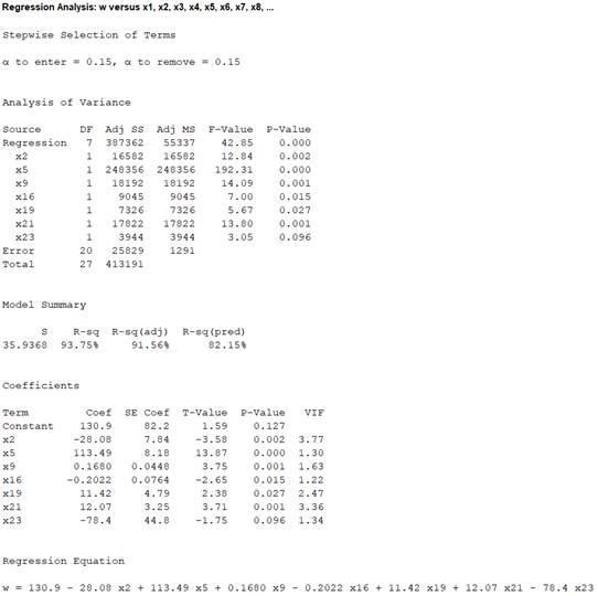
The ‘Coefficient’ column of the regression analysis MINITAB output gives the slopes corresponding to the respective variables stored in the column ‘Term’.

A careful inspection of the output shows that the fitted model is:

$\widehat{w}=\left(\begin{array}{l}130.9-28.08x_2+113.49x_5+0.1680x_9-0.2022x_{16}\\ +11.42x_{19}+12.07x_{21}-78.4x_{23}\end{array}\right)$.

Hence, the regression equation to predict w using the stepwise regression method is:

$\underset{\_}{\widehat{w}=\left(\begin{array}{l}130.9-28.08x_2+113.49x_5+0.1680x_9-0.2022x_{16}\\ +11.42x_{19}+12.07x_{21}-78.4x_{23}\end{array}\right)}$.

If the P-value of the predictor variable is greater than the level of significance, there is no significant effect of the predictor variable and one can drop the variable.

Now, according to the MINITAB output the P-value of $X_{16}$, $X_{19}$ and $X_{23}$ are 0.015, 0.027 and 0.096, respectively.

Those P-values are greater than the respective level of significance 0.05.

Hence, it is reasonable to drop the variables $X_{16}$, $X_{19}$ and $X_{23}$.