
Concept explainers
Videos
a.
Find the 95% confidence interval for the slope of Manganese.
a.
Answer to Problem 2E
The 95% confidence interval for the slope of Manganese is
Explanation of Solution
Given info:
The data represents the MINITAB output of the regression model
Calculation:
Multiple linear regression model:
A multiple linear regression model is given as
The ‘Coefficient’ column of the regression analysis MINITAB output gives the slopes corresponding to the respective variables stored in the column ‘Predictor’.
Let
From the accompanying MINITAB output, the slope coefficient of Manganese is
Confidence interval:
The general formula for the confidence interval for the slope of the regression line is,
Where,
From the accompanying MINITAB output, the estimate of error standard deviation of slope coefficient of Manganese is
Critical value:
For 95% confidence level,
Degrees of freedom:
The number of plates that are sampled is
The degrees of freedom is,
From Table A.5 of the t- distribution in Appendix A, the critical value corresponding to the right tail area 0.025 and 17 degrees of freedom is 2.110.
Thus, the critical value is
The 95% confidence interval is,
Thus, the 95% confidence interval for the slope of Manganese is
Interpretation:
There is 95% confident that the average change in the tensile strength associated with 1 ppt increase in manganese lies between
b.
Find the 99% confidence interval for the slope of Thickness.
b.
Answer to Problem 2E
The 99% confidence interval for the slope of Thickness is
Explanation of Solution
Calculation:
From the accompanying MINITAB output, the slope coefficient of Thickness is
Confidence interval:
The general formula for the confidence interval for the slope of the regression line is,
Where,
From the accompanying MINITAB output, the estimate of error standard deviation of slope coefficient of Thickness is
Critical value:
For 99% confidence level,
Degrees of freedom:
The number of plates that are sampled is
The degrees of freedom is,
From Table A.5 of the t- distribution in Appendix A, the critical value corresponding to the right tail area 0.005 and 17 degrees of freedom is 2.898.
Thus, the critical value is
The 95% confidence interval is,
Thus, the 99% confidence interval for the slope of Thickness is
Interpretation:
There is 99% confident that the average change in the tensile strength associated with 1 ppt increase in Thickness lies between
c.
Test whether there is enough evidence to conclude that
c.
Answer to Problem 2E
There is no sufficient evidence to conclude that
Explanation of Solution
Calculation:
From the accompanying MINITAB output, the slope coefficient of Manganese is
Here, the claim is that
The test hypotheses are given below:
Null hypothesis:
That is, 1 ppt increase in manganese tends to at most
Alternative hypothesis:
That is, increase in the true average of tensile strength due to 1 ppt increase in manganese will be greater than
Test statistic:
The test statistic is,
Where,
From the accompanying MINITAB output, the estimate of error standard deviation of slope coefficient of Manganese is
Test statistic under null hypothesis:
Under the null hypothesis, the test statistic is obtained as follows:
Thus, the test statistic is 0.9642.
Degrees of freedom:
The number of plates that are sampled is
The degrees of freedom is,
Thus, the degree of freedom is 17.
Here, level of significance is not given.
So, the prior level of significance
P-value:
Software procedure:
Step by step procedure to obtain the P- value using the MINITAB software:
- Choose Graph > Probability Distribution Plot choose View Probability > OK.
- From Distribution, choose ‘t’ distribution and enter 17 as degrees of freedom.
- Click the Shaded Area tab.
- Choose X-Value and Right Tail for the region of the curve to shade.
- Enter the X-value as 0.9642.
- Click OK.
Output obtained from MINITAB is given below:
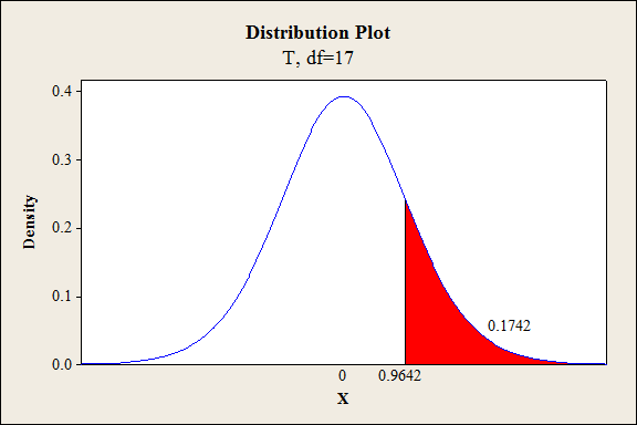
From the output, the P- value is 0.1742.
Thus, the P- value is 0.1742.
Decision criteria based on P-value approach:
If
If
Conclusion:
The P-value is 0.1742 and
Here, P-value is greater than the
That is
By the rejection rule, fail to reject the null hypothesis.
Hence, 1 ppt increase in manganese tends to at most
Therefore, there is no sufficient evidence to conclude that
d.
Test whether there is enough evidence to conclude that
d.
Answer to Problem 2E
There is sufficient evidence to conclude that
Explanation of Solution
Calculation:
From the accompanying MINITAB output, the slope coefficient of Thickness is
Here, the claim is that
The test hypotheses are given below:
Null hypothesis:
That is, 1 mm increase in thickness tends to at least
Alternative hypothesis:
That is, decrease in the true average of tensile strength due to 1 mm increase in thickness will be less than
Test statistic:
The test statistic is,
Where,
From the accompanying MINITAB output, the estimate of error standard deviation of slope coefficient of Thickness is
Test statistic under null hypothesis:
Under the null hypothesis, the test statistic is obtained as follows:
Thus, the test statistic is -2.577.
Degrees of freedom:
The number of plates that are sampled is
The degrees of freedom is,
Thus, the degree of freedom is 17.
Here, level of significance is not given.
So, the prior level of significance
P-value:
Software procedure:
Step by step procedure to obtain the P- value using the MINITAB software:
- Choose Graph > Probability Distribution Plot choose View Probability > OK.
- From Distribution, choose ‘t’ distribution and enter 17 as degrees of freedom.
- Click the Shaded Area tab.
- Choose X-Value and Left Tail for the region of the curve to shade.
- Enter the X-value as -2.577.
- Click OK.
Output obtained from MINITAB is given below:
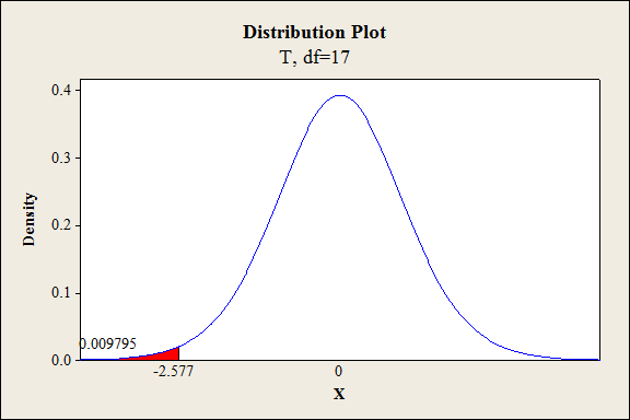
From the output, the P- value is 0.009795.
Thus, the P- value is 0.009795.
Decision criteria based on P-value approach:
If
If
Conclusion:
The P-value is 0.009795 and
Here, P-value is less than the
That is
By the rejection rule, reject the null hypothesis.
Hence, 1 mm increase in thickness tends to at least
Therefore, there is sufficient evidence to conclude that
Want to see more full solutions like this?
Chapter 8 Solutions
Statistics for Engineers and Scientists


- A 95% confidence interval for the proportion of U.S. adults who subscribe to some sort of streaming service is (0.685, 0.745). The point estimate for this confidence interval is: A. 0.060 B. 0.044 C. 0.030 D. 0.715arrow_forwardA statistics student wants to conduct a study to determine the proportion of workers in Cititon who commute to another town for work. If the student wants a 90% confidence interval with a margin of error of 2%, how many workers should be in her sample?arrow_forwardIn practice, if we don’t know whether the population is normal and our sample size is less than 30, when can we proceed with inference for confidence intervals and hypothesis testing? a)When α is set very low b)When the number of successes exceeds the number of failures c)When the sample standard deviation is not large d)When the data is single-peaked and there are no outliersarrow_forward
- 4. Ten students on a low-fat diet designed to lower their cholesterol and recorded their before and after diet data in the following table: Before diet cholesterol level: After diet cholesterol level: 140 140 220 230 110 120 240 220 200 190 180 150 190 200 360 300 280 300 260 240 Based on a 95% confidence level, after hypothesis testing, what would you tell the students about the diet? Does the null hypothesis reject H0 or fail to reject H0?arrow_forwardIn a study of the accuracy of fast food drive-through orders, Restaurant A had 307 accurate orders and 64 that were not accurate. a. Construct a 90% confidence interval estimate of the percentage of orders that are not accurate. b. Compare the results from part (a) to this 90% confidence interval for the percentage of orders that are not accurate at Restaurant B: 0.161<p<0.222. What do you conclude?arrow_forwardwo groups of men, those dressed as Luke Skywalker and those dressed as storm troopers were measured for height in inches. Data in table below: Lukes Storm Troopers xbar=67 xbar = 70 n=14 n=11 sd = 1 sd = 3 Using this data, and the assumption that the population variances are equal, give a 90% confidence interval for mu (storm troopers) - mu (lukes) = μS - μLarrow_forward
- 5. A phase three clinical trial for a new medication proposed to treat depression has 1191 participants. If all these individuals are from the group of individuals who were given the medication and 759 individuals who received the medication experienced improvement in their symptoms of depression, construct a 90% confidence interval for the true proportion of individuals on the medication who experienced improvement in their symptoms of depression.A) (.363, .417)B) (.335, .363)C) (.623, .651)D) (.614, .660)arrow_forwardIn a situation where the sample size was decreased from 39 to 29 in a normally distributed data set, what would be the impact on the confidence interval?arrow_forwardA medical survey in 2015 indicated that 48% of Australian adults prefer to take a generic drug than pay more for a name brand equivalent. A pharmaceutical company believes that with the financial crisis, the percentage of Australian adults willing to take a cheaper generic drug may have risen. The research department conducted a study where a random sample of Australian adults were asked whether or not they would accept a cheaper generic prescription drug. a) What type of hypothesis test would be appropriate to investigate the pharmaceutical company’s prediction? (b) What is the population we can draw conclusions about in this study? (c) The appropriate hypothesis test was conducted and a p-value of .110 was obtained. Based on the results of this study, the pharmaceutical company concludes that the percentage of Australian adults willing to take a cheaper generic prescription drug has remained the same, exactly 48%. Comment on the validity of this conclusion. Provide justification…arrow_forward
- In an article in the Journal of Advertising, Weinberger and Spotts compare the use of humor in television ads in the United States and the United Kingdom. They found that a substantially greater percentage of U.K. ads use humor.a. Suppose that a random sample of 400 television ads in the United Kingdom reveals that 142 of these ads use humor. Find a point estimate of and a 95 percent confidence interval for the proportion of all U.K. television ads that use humor.b. Suppose a random sample of 500 television ads in the United States reveals that 122 of these ads use humor. Find a point estimate of and a 95 percent confidence interval for the proportion of all U.S. television ads that use humor.c. Do the confidence intervals you computed in parts a and b suggest that a greater percentage of U.K. ads use humor? Explain.arrow_forwardIn a study of the accuracy of fast food drive-through orders, Restaurant A had 290 accurate orders and 56 that were not accurate. a. Construct a 90% confidence interval estimate of the percentage of orders that are not accurate. b. Compare the results from part (a) to this 90% confidence interval for the percentage of orders that are not accurate at Restaurant B: 0.146 <p < 0.212. What do you conclude?arrow_forwardIn testing hypotheses, which of the following would be strong evidence against the null hypothesis?a. Obtaining data with a test statistic of small magnitude.b. Obtaining data with a small P-value.c. Obtaining data with a large P-value.d. Using a large level of significance, α.e. Using a small level of significance, αarrow_forward
 MATLAB: An Introduction with ApplicationsStatisticsISBN:9781119256830Author:Amos GilatPublisher:John Wiley & Sons Inc
 Probability and Statistics for Engineering and th...StatisticsISBN:9781305251809Author:Jay L. DevorePublisher:Cengage Learning
 Statistics for The Behavioral Sciences (MindTap C...StatisticsISBN:9781305504912Author:Frederick J Gravetter, Larry B. WallnauPublisher:Cengage Learning
 Elementary Statistics: Picturing the World (7th E...StatisticsISBN:9780134683416Author:Ron Larson, Betsy FarberPublisher:PEARSON
 The Basic Practice of StatisticsStatisticsISBN:9781319042578Author:David S. Moore, William I. Notz, Michael A. FlignerPublisher:W. H. Freeman
 Introduction to the Practice of StatisticsStatisticsISBN:9781319013387Author:David S. Moore, George P. McCabe, Bruce A. CraigPublisher:W. H. Freeman