
Videos
The article “Combined Analysis of Real-Time Kinematic GPS Equipment and Its Users for Height Determination” (W. Featherstone and M. Stewart, Journal of Surveying Engineering. 2001:31–51) presents a study of the accuracy of global positioning system (GPS) equipment in measuring heights. Three types of equipment were studied, and each was used to make measurements at four different base stations (in the article a fifth station was included, for which the results differed considerably from the other four). There were 60 measurements made with each piece of equipment at each base. The means and standard deviations of the measurement errors (in mm) are presented in the following table for each combination of equipment type and base station.
- a. Construct an ANOVA table. You may give
ranges for the P-values. - b. The question of interest is whether the mean error differs among instruments. It is not of interest to determine whether the error differs among base stations. For this reason, a surveyor suggests treating this as a randomized complete block design, with the base stations as the blocks. Is this appropriate? Explain.
a.
Construct the ANOVA.
Answer to Problem 9SE
The ANOVA table is,
| Source | DF | SS | MS | F | P |
| Base | 3 | 13,495 | 4498.3 | 7.5308 | 0.000 |
| Instrument | 2 | 90,990 | 45,495 | 76.164 | 0.000 |
| Interaction | 6 | 12,050 | 2,008.3 | 3.3622 | 0.003 |
| Error | 708 | 422,912 | 597.33 | ||
| Total | 719 | 539,447 |
Explanation of Solution
Calculation:
The given information is based on the accuracy of the global positioning system (GPS) which has 3 instruments that have to make measurements at four different base stations have 60 measurements with each piece of instrument at each base.
Let us denote the main effects of Instruments (I) with
The aim is to find the ANOVA.
State the hypothesis:
Main effect of Instruments:
Null hypothesis:
Alternative hypothesis:
Main effect of Base:
Null hypothesis:
Alternative hypothesis:
Interaction:
Null hypothesis:
Alternative hypothesis:
ANOVA table:
| Source | DF | SS | MS | F |
| Treatment | ||||
| Blocks | ||||
| Interaction | ||||
| Error | ||||
| Total |
Where,
Where, N is the sample size, I denotes the number of treatments,
Here, the number of treatments (I) is 3, the number of blocks (J) is 4 and the number of replicates (K) is 60.
Test the hypothesis on 5% level of significance:
Here, Instrument is the treatments and Base is the blocks.
Level of significance:
The level of significance is
Degrees of freedom:
Base degrees of freedom:
Instrument degrees of freedom:
Interaction degrees of freedom:
Error degrees of freedom:
Total degrees of freedom:
The treatment and block means are tabulated below:
| Base | Instruments | Block mean | ||
| Instrument A | Instrument B | Instrument C | ||
| 0 | 3 | –24 | –6 | –9 |
| 1 | 14 | –13 | –2 | –0.33 |
| 2 | 1 | –22 | 4 | –5.667 |
| 3 | 8 | –17 | 15 | 2 |
| Treatment mean | 6.5 | –19 | 2.75 | |
By observing the data, the values of
For Base:
The value of SSB (Base) is:
Substitute
The value of MSB (Base) is:
Substitute
For Instruments:
The value of SSTr ( Instruments) is:
Substitute
The value of MSTr (Instruments) is:
Substitute
For Interaction Factor (AB):
The value of SSAB is:
Substitute
The value of MSAB is:
Substitute
The value of MSE is:
Substitute
The value of SSE is:
The value of SST is:
The value of F statistic is:
For Base:
Substitute
Thus, the value of F statistic for Base is 7.5308.
For Instruments:
Substitute
Thus, the value of F statistic for Instruments is 76.164.
For Interaction factor (AB):
Substitute
Thus, the value of F statistic for interaction is 3.3622.
The ranges of P-values are:
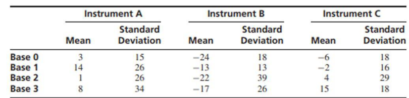
For Base
Software procedure:
Step by step procedure to obtain the critical-value using the MINITAB software is given below:
- Choose Graph > Probability Distribution Plot choose View Probability> OK.
- From Distribution, choose ‘F’ distribution.
- Enter Numerator Df as 3.
- Enter Denominator Df as 708.
- Click the Shaded Area tab.
- Choose X Value and Right Tail for the region of the curve to shade.
- Enter the Data value as 7.5308.
- Click OK.
Output using the MINITAB software is given below:
From the MINITAB output, the value of
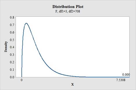
For Instruments
Software procedure:
Step by step procedure to obtain the critical-value using the MINITAB software is given below:
- Choose Graph > Probability Distribution Plot choose View Probability> OK.
- From Distribution, choose ‘F’ distribution.
- Enter Numerator Df as 2.
- Enter Denominator Df as 708.
- Click the Shaded Area tab.
- Choose X Value and Right Tail for the region of the curve to shade.
- Enter the Data value as 76.164.
- Click OK.
Output using the MINITAB software is given below:
From the MINITAB output, the value of
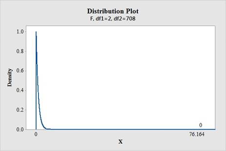
For interaction
Software procedure:
Step by step procedure to obtain the critical-value using the MINITAB software is given below:
- Choose Graph > Probability Distribution Plot choose View Probability> OK.
- From Distribution, choose ‘F’ distribution.
- Enter Numerator Df as 6.
- Enter Denominator Df as 708.
- Click the Shaded Area tab.
- Choose X Value and Right Tail for the region of the curve to shade.
- Enter the Data value as 3.3622.
- Click OK.
Output using the MINITAB software is given below:
From the MINITAB output, the value of
The ANOVA table is,
| Source | DF | SS | MS | F | P |
| Base | 3 | 13,495 | 4498.3 | 7.5308 | 0.000 |
| Instrument | 2 | 90,990 | 45,495 | 76.164 | 0.000 |
| Interaction | 6 | 12,050 | 2,008.3 | 3.3622 | 0.003 |
| Error | 708 | 422,912 | 597.33 | ||
| Total | 719 | 539,447 |
Conclusion:
Base (Block):
Here, the P-value is less than the level of significance.
That is,
Therefore, the null hypothesis is rejected.
Thus, it can be concluded that there is a significant difference between block effects.
Instrument (Treatment):
Here, the P-value is less than the level of significance.
That is,
Therefore, the null hypothesis is rejected.
Thus, it can be concluded that there is a significant difference between treatment effects.
Interaction:
Here, the P-value is less than the level of significance.
That is,
Therefore, the null hypothesis is rejected.
Thus, it can be concluded that there is a significant effect of the interaction between the base (block) and instrument (treatment).
b.
Decide whether it is appropriate to treat the randomized complete block design with base stations as blocks to determine the interest that the mean error differs among the instruments.
Answer to Problem 9SE
No, it is not appropriate to treat the data with a randomized complete block design with base stations as blocks.
Explanation of Solution
In randomized complete block design, there must be no the interaction between the treatment factor and the blocking factor, so that the treatment factor may be interpreted in RBD. However, here, the interaction effect is significant, suggesting that it is not possible to use randomized complete block design.
Thus, the suggestion given by the surveyor to treat the randomized complete block design with base station as blocks is not appropriate.
Want to see more full solutions like this?
Chapter 9 Solutions
Statistics for Engineers and Scientists
Additional Math Textbook Solutions
Statistical Techniques in Business and Economics
Fundamentals of Statistics (5th Edition)
Statistical Reasoning for Everyday Life (5th Edition)
An Introduction to Mathematical Statistics and Its Applications (6th Edition)
APPLIED STAT.IN BUS.+ECONOMICS
Elementary Statistics (13th Edition)


- In a study attempting to replicate findings by Stephens, Atkins, & Kingston (2009), each participant was asked to plunge a hand into the icy water and keep it there as long as the pain would allow. In one condition, the participants repeated their favorite curse words while their hands were in the water. In the other condition, they repeated neutral words. The original research showed that, in addition to lowering the participants’ perception of pain, swearing also increased the amount of time they were able to tolerate the pain. Data similar to the results obtained in the study are shown in the following table: _____________Amount of Time (in Seconds)_ Participant Swear Words Neutral Words 1 94 59 2 70 61 3 52 47 4…arrow_forwardA paper investigated the driving behavior of teenagers by observing their vehicles as they left a high school parking lot and then again at a site approximately 1 2 mile from the school. Assume that it is reasonable to regard the teen drivers in this study as representative of the population of teen drivers. MaleDriver FemaleDriver 1.4 -0.2 1.2 0.5 0.9 1.1 2.1 0.7 0.7 1.1 1.3 1.2 3 0.1 1.3 0.9 0.6 0.5 2.1 0.5 (a) Use a .01 level of significance for any hypothesis tests. Data consistent with summary quantities appearing in the paper are given in the table. The measurements represent the difference between the observed vehicle speed and the posted speed limit (in miles per hour) for a sample of male teenage drivers and a sample of female teenage drivers. (Use ?males − ?females. Round your test statistic to two decimal places. Round your degrees of freedom down to the nearest whole number. Round your p-value to three decimal places.) t = df =…arrow_forwardA paper investigated the driving behavior of teenagers by observing their vehicles as they left a high school parking lot and then again at a site approximately 1 2 mile from the school. Assume that it is reasonable to regard the teen drivers in this study as representative of the population of teen drivers. MaleDriver FemaleDriver 1.3 -0.3 1.3 0.6 0.9 1.1 2.1 0.7 0.7 1.1 1.3 1.2 3 0.1 1.3 0.9 0.6 0.5 2.1 0.5 (a) Use a .01 level of significance for any hypothesis tests. Data consistent with summary quantities appearing in the paper are given in the table. The measurements represent the difference between the observed vehicle speed and the posted speed limit (in miles per hour) for a sample of male teenage drivers and a sample of female teenage drivers. (Use ?males − ?females. Round your test statistic to two decimal places. Round your degrees of freedom down to the nearest whole number. Round your p-value to three decimal places.) t = df =…arrow_forward
- Question Two A Deputy Registrar at a certainty university conducted a Chi-Square test of association to establish whether or not employee grade and level of absenteeism were associated. Table 2 below shows part of the results which were obtained. Table 2: Cross tabulation of employee grade and level of absenteeism Contingency Tables Grade LAbsence 1 2 3 Total low Observed 8 1 0 9 Expected 2.90 3.48 2.61 9.00 high Observed 2 11 9 22 Expected 7.10 8.52 6.39 22.00 Total Observed 10 12 9 31 Expected 10.00 12.00 9.00 31.00 2.1 State the appropriate measurement scales for the variables. 2.2 State the null and alternative hypotheses. 2.3 Calculate the expected frequency corresponding to a Grade 3 academic with a high level of absenteeism. 2.4 Find the Chi-Square critical value and test…arrow_forwardCompare the two separate scatterplots. In particular, how do the associtation compare between women with pets vs. women without pets? Does one group have more variation in systolic blood pressure than the other? If so, for which group? Does systolic blood pressure seem higher for common ages between the two groups? If so, for which group?arrow_forwardQuestion 2 A researcher was interested in studying if there is a significant relationship between the severity of COVID 19 and blood types of individuals. 2400 individuals were studied and the results are shown below. Condition Blood Type O A B AB Total Critical 64 44 20 8 136 Severe 175 129 50 15 369 Moderate 211 528 151 125 1015 Mild 200 400 140 140 880 Total 650 1101 361 288 240 a .State both the null and alternative hypotheses. b. Provide the decision rule for making this decision. Use an alpha level of 5%. c. Show all of the work necessary to calculate the appropriate statistic.d. What conclusion are you allowed to draw? e. Would your conclusion change at the 10% level of significance?arrow_forward
- given this data, what will be the most appropriate way to present them?arrow_forwardIn the COVID-19 data set, there are several questions that participants answer about the reactions of their government to the pandemic, as well as questions about their own well-being, in terms of measures of distress, such as anxiety and depression. This data was collected quite early in the pandemic, near the beginning of the first wave in late March. One might ask whether how one viewed their government might affect one's concerns about the health of their family and themselves. What type of procedure might you use to see whether there was an association between attitudes towards governtment and worries about health? Group of answer choices Correlation Related Samples t Test Chi-Square Goodness of Fit Test Oneway ANOVAarrow_forwardIn a classic study, Shrauger (1972) examined the effect of an audience on performance for two groups of participants: high self-esteem and low self-esteem individuals. The participants in the study were given a problem-solving task with half of the individuals in each group working alone and a half working with an audience. Performance on the problem-solving task was measured for each individual. The results showed that the presence of an audience had little effect on high self-esteem participants but significantly lowered the performance for the low self-esteem participants. a. How many factors does this study have? What are they? b. Describe this study using the notation system that indicates factors and numbers of levels of each factor.arrow_forward
- determine the following statement is a valid reason for using nonparametric methods? - We are reluctant to assume strong conditions on the data. (True or False)arrow_forwardConsider a cohort study to compare the mortality rate of myocardial infarction (MI) in men with sedentary work (exposed group) to men with physically active work (unexposed). If in the exposed, there were 36,000 person (man) years of observation and 126 deaths whereas the unexposed had 24,000 man-years of observation and 44 deaths. Compute the following a) Mortality rate in each cohort? b) What is the relative risk of dying, comparing these 2 groups? c) What is the attributable risk of sedentary work? d) What is the attributable benefit of physical activity? e) If we assume that MI is associated with the mortality in this cohort (causality), what proportion of the disease in the higher group is potentially preventable?arrow_forwardrofessor Cornish studied rainfall cycles and sunspot cycles. (Reference: Australian Journal of Physics, Vol. 7, pp. 334-346.) Part of the data include amount of rain (in mm) for 6-day intervals. The following data give rain amounts for consecutive 6-day intervals at Adelaide, South Australia. 7 28 7 1 69 3 1 4 22 7 16 4 54 160 60 73 27 3 3 1 7 144 107 4 91 44 1 8 4 22 4 59 116 52 4 155 42 24 11 43 3 24 19 74 26 63 110 39 34 71 52 39 8 0 15 2 14 9 1 2 4 9 6 10 (i) Find the median. (Use 1 decimal place.)(ii) Convert this sequence of numbers to a sequence of symbols A and B, where A indicates a value above the median and B a value below the median. Test the sequence for randomness about the median at the 5% level of significance. (b) Find the number of runs R, n1, and n2. Let n1 = number of values above the median and n2 = number of values below the median. R n1 n2 (c) In the case, n1 > 20, we cannot use Table 10 of Appendix II to find the critical…arrow_forward
 MATLAB: An Introduction with ApplicationsStatisticsISBN:9781119256830Author:Amos GilatPublisher:John Wiley & Sons Inc
 Probability and Statistics for Engineering and th...StatisticsISBN:9781305251809Author:Jay L. DevorePublisher:Cengage Learning
 Statistics for The Behavioral Sciences (MindTap C...StatisticsISBN:9781305504912Author:Frederick J Gravetter, Larry B. WallnauPublisher:Cengage Learning
 Elementary Statistics: Picturing the World (7th E...StatisticsISBN:9780134683416Author:Ron Larson, Betsy FarberPublisher:PEARSON
 The Basic Practice of StatisticsStatisticsISBN:9781319042578Author:David S. Moore, William I. Notz, Michael A. FlignerPublisher:W. H. Freeman
 Introduction to the Practice of StatisticsStatisticsISBN:9781319013387Author:David S. Moore, George P. McCabe, Bruce A. CraigPublisher:W. H. Freeman