4. Use a third order polynomial approximation of s(t) to approximate the velocity at t=30s using a. Direct Fit Polynomial Method b. Lagrange Polynomial Method
4. Use a third order polynomial approximation of s(t) to approximate the velocity at t=30s using a. Direct Fit Polynomial Method b. Lagrange Polynomial Method

Functions and Change: A Modeling Approach to College Algebra (MindTap Course List)
6th Edition
ISBN:9781337111348
Author:Bruce Crauder, Benny Evans, Alan Noell
Publisher:Bruce Crauder, Benny Evans, Alan Noell
Chapter2: Graphical And Tabular Analysis
Section2.1: Tables And Trends
Problem 1TU: If a coffee filter is dropped, its velocity after t seconds is given by v(t)=4(10.0003t) feet per...

Related questions
Question
100%
pls help me with number 4 thank you
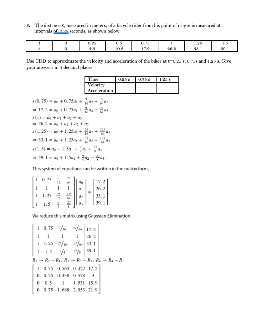
Transcribed Image Text:The distance s, measured in meters, of a bicycle rider from his point of origin is measured at
intervals of 0 25 seconds, as shown below
3.
0.25
0.5
0.75
1.25
1.5
4.3
10.2
17.2
26.2
33.1
39.1
Use CDD to approximate the velocity and acceleration of the biker at t=0.25 s, 0.75s and 1.25 s. Give
your answers in 4 decimal places.
Time
Velocity
Acceleration
0.25 s
0.75 s
1.25 s
s (0. 75) = ao + 0. 75a, + a2 + az
= 17.2 = ao + 0.75a + az + az
1642
s (1) = ao + aj + az + az
> 26. 2 = ao + aị + a2 + az
25
s (1. 25) = ao + 1. 25ai + a2 +
= 33. 1 = ao + 1. 25a, + a
1642 +
125
64 a3
s (1.5) = ao + 1. 5a1 + a2 + az
= 39.1 = ao + 1. 5a1 + a2 + az.
This system of equations can be written in the matrix form,
1 0.75
17.2
1
1
1
1
26. 2
1
1. 25 25
125
33. 1
a2
64
1
1.5
39. 1
We reduce this matrix using Gaussian Elimination,
1 0.75 /16 27/64 17.2
1
1
1
1
26. 2
1 1.25 25/16 125/64 33. 1
1 1.5 4 27/s 39. 1
R2 → R2 – R1, R3 → R3 – R1, R4 → R4 – R1
1 0. 75 0. 563 0.422 17. 2
0 0. 25 0.438 0. 578
9
1. 531 15.9
0 0. 75 1.688 2.953 21.9
0 0.5
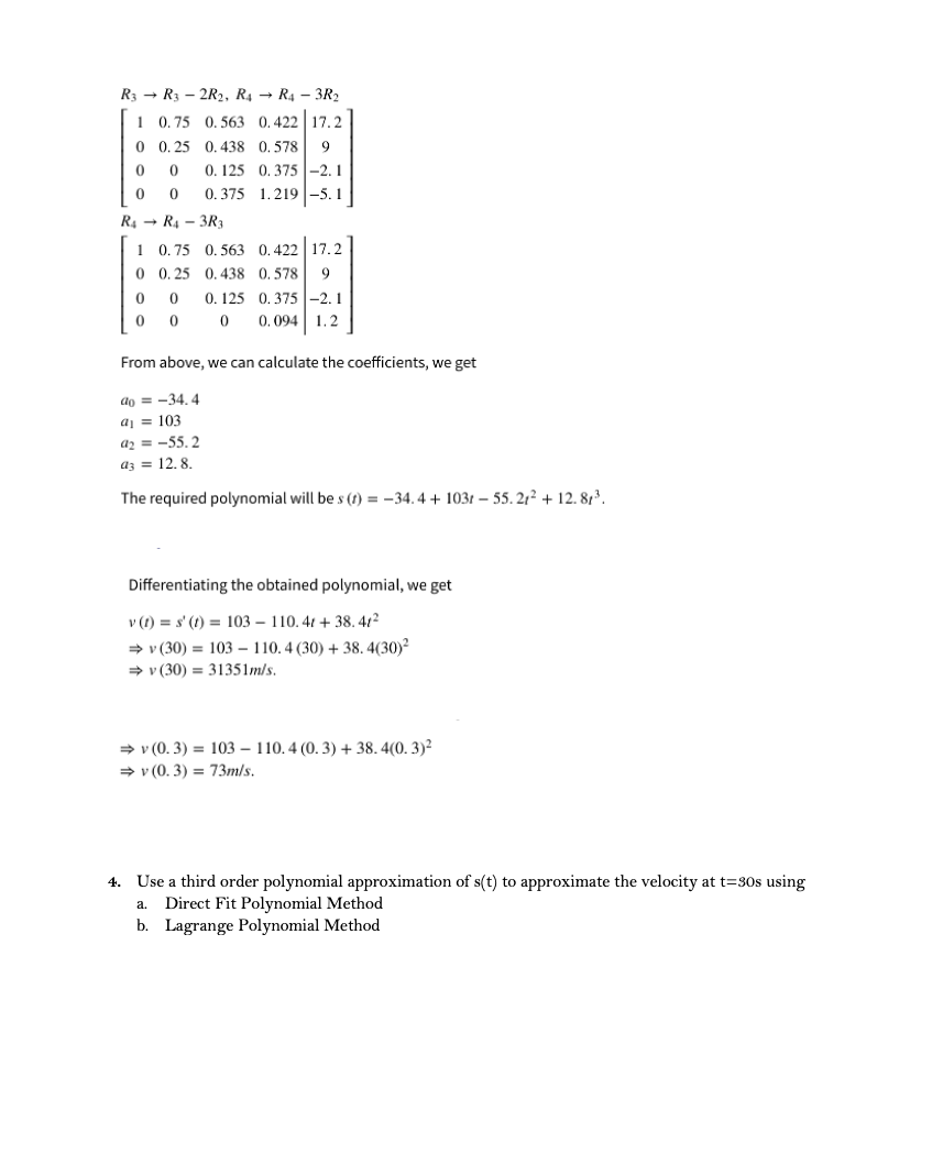
Transcribed Image Text:R3 → R3 – 2R2, R4 → R4 – 3R2
1 0.75 0. 563 0.422 17.2
0 0. 25 0. 438 0. 578
9
0. 125
0. 375 -2.1
0. 375 1.219 -5.1
R4 - R4 - 3R3
1 0.75 0. 563 0, 422 | 17.2
0 0. 25 0.438 0. 578
0. 125 0.375|-2.1
0.094 1.2
From above, we can calculate the coefficients, we get
do = -34. 4
aj = 103
az = -55.2
az = 12. 8.
The required polynomial will be s (1) = -34. 4 + 1031 – 55. 21² + 12. 8,3.
Differentiating the obtained polynomial, we get
v (1) = s' (1) = 103 – 110. 41 + 38. 412
+ v (30) = 103 – 110. 4 (30) + 38. 4(30)?
> v (30) = 31351m/s.
→ v (0. 3) = 103 – 110.4 (0. 3) + 38. 4(0. 3)²
→ v (0. 3) = 73m/s.
4. Use a third order polynomial approximation of s(t) to approximate the velocity at t=30s using
Direct Fit Polynomial Method
b. Lagrange Polynomial Method
a.
Expert Solution
This question has been solved!
Explore an expertly crafted, step-by-step solution for a thorough understanding of key concepts.

Step by step
Solved in 4 steps

Recommended textbooks for you
Functions and Change: A Modeling Approach to Coll…
Algebra
ISBN:
9781337111348
Author:
Bruce Crauder, Benny Evans, Alan Noell
Publisher:
Cengage Learning

Algebra & Trigonometry with Analytic Geometry
Algebra
ISBN:
9781133382119
Author:
Swokowski
Publisher:
Cengage

Trigonometry (MindTap Course List)
Trigonometry
ISBN:
9781337278461
Author:
Ron Larson
Publisher:
Cengage Learning
Functions and Change: A Modeling Approach to Coll…
Algebra
ISBN:
9781337111348
Author:
Bruce Crauder, Benny Evans, Alan Noell
Publisher:
Cengage Learning
Algebra & Trigonometry with Analytic Geometry
Algebra
ISBN:
9781133382119
Author:
Swokowski
Publisher:
Cengage
Trigonometry (MindTap Course List)
Trigonometry
ISBN:
9781337278461
Author:
Ron Larson
Publisher:
Cengage Learning
