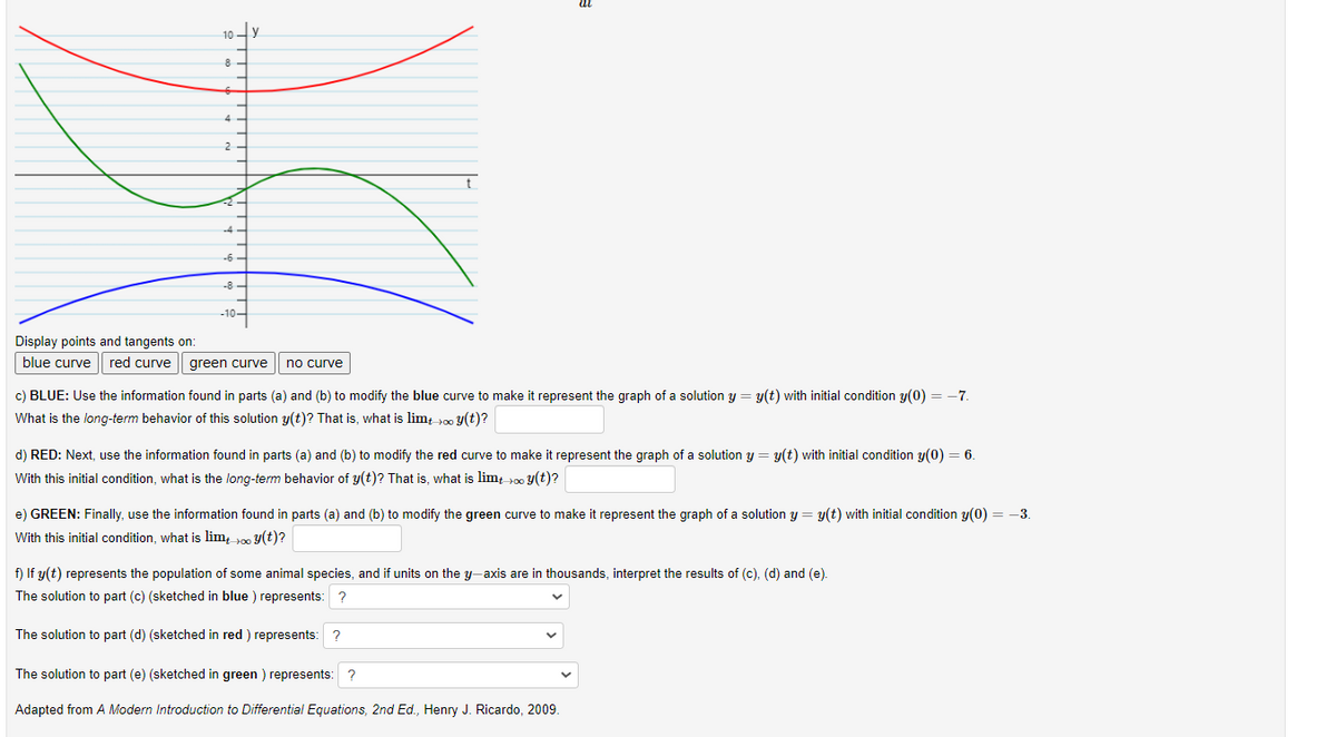
Even before you learn techniques for solving differential equations, you may be able to analyze equations qualitatively. As an example, look at the nonlinear equation dy (y – 4)°(y + 5) dt You are going to analyze the solutions, y, of this equation without actually finding them. You will be asked to sketch three solutions of the differential equation on the graph below based on qualitative informat differential equation. In what follows, picture the t-axis running horizontally and the y axis running vertically. There is no scale on the t axis but imagine it is large enough to display the behavior of the solutions as t approaches + a) For what values of y is the graph of y as a function of t increasing? Use interval notation for your answer. (-5,4)U(4,INF) b) For what values of y is the graph of y concave up? (-INF,-5)U(4,INF) For what values of y is it concave down? (-INF.-4)U(-2,4) (Help with interval notation.) What information do you need to answer question about concavity? Remember that y is an implicit function of t. (How to enter answer] Parts c),d), e) of this question ask you to modify the blue, red, and green curves in the plot below to make them represent graphs of particular solutions of the differential equation, To modify the blue curve, click the "blue curve" button below the plot to expose blue points and tangents. Solid blue points lie on the curve. With your mouse click and hold each solid blue point, and move it i position. If the solution curve crosses an edge of the viewing region then the corresponting solid point should be very near the edge, left or right, top or bottom. Improve the shape of the curve between the so moving the open points that lie on the dashed tangents. Experiment to see how the shape changes. Modify the red or green curve in a similar way, after clicking the corresponding button to expose its points and tangents. I recommend moving solid points into good positions first, then move the open points shape between the solid points. dy = (y – 4)°(y + 5). 4.
Even before you learn techniques for solving differential equations, you may be able to analyze equations qualitatively. As an example, look at the nonlinear equation dy (y – 4)°(y + 5) dt You are going to analyze the solutions, y, of this equation without actually finding them. You will be asked to sketch three solutions of the differential equation on the graph below based on qualitative informat differential equation. In what follows, picture the t-axis running horizontally and the y axis running vertically. There is no scale on the t axis but imagine it is large enough to display the behavior of the solutions as t approaches + a) For what values of y is the graph of y as a function of t increasing? Use interval notation for your answer. (-5,4)U(4,INF) b) For what values of y is the graph of y concave up? (-INF,-5)U(4,INF) For what values of y is it concave down? (-INF.-4)U(-2,4) (Help with interval notation.) What information do you need to answer question about concavity? Remember that y is an implicit function of t. (How to enter answer] Parts c),d), e) of this question ask you to modify the blue, red, and green curves in the plot below to make them represent graphs of particular solutions of the differential equation, To modify the blue curve, click the "blue curve" button below the plot to expose blue points and tangents. Solid blue points lie on the curve. With your mouse click and hold each solid blue point, and move it i position. If the solution curve crosses an edge of the viewing region then the corresponting solid point should be very near the edge, left or right, top or bottom. Improve the shape of the curve between the so moving the open points that lie on the dashed tangents. Experiment to see how the shape changes. Modify the red or green curve in a similar way, after clicking the corresponding button to expose its points and tangents. I recommend moving solid points into good positions first, then move the open points shape between the solid points. dy = (y – 4)°(y + 5). 4.

Calculus: Early Transcendentals
8th Edition
ISBN:9781285741550
Author:James Stewart
Publisher:James Stewart
Chapter1: Functions And Models
Section: Chapter Questions
Problem 1RCC: (a) What is a function? What are its domain and range? (b) What is the graph of a function? (c) How...

Related questions
Question
Transcribed Image Text:10-
4
2
-6-
-8 -
-10-
Display points and tangents on:
blue curve | red curve || green curve
no curve
c) BLUE: Use the information found in parts (a) and (b) to modify the blue curve to make it represent the graph of a solution y = y(t) with initial condition y(0) = -7.
What is the long-term behavior of this solution y(t)? That is, what is lim0 Y(t)?
d) RED: Next, use the information found in parts (a) and (b) to modify the red curve to make it represent the graph of a solution y = y(t) with initial condition y(0) = 6.
With this initial condition, what is the long-term behavior of y(t)? That is, what is lim 00 y(t)?
e) GREEN: Finally, use the information found in parts (a) and (b) to modify the green curve to make it represent the graph of a solution y = y(t) with initial condition y(0) = -3.
With this initial condition, what is lim, 0 y(t)?
f) If y(t) represents the population of some animal species, and if units on the y-axis are in thousands, interpret the results of (c), (d) and (e).
The solution to part (c) (sketched in blue ) represents: ?
The solution to part (d) (sketched in red ) represents: ?
The solution to part (e) (sketched in green ) represents: ?
Adapted from A Modern Introduction to Differential Equations, 2nd Ed., Henry J. Ricardo, 2009.
![Even before you learn techniques for solving differential equations, you may be able to analyze equations qualitatively . As an example, look at the nonlinear equation
dy
(y – 4)°(y + 5)
dt
You are going to analyze the solutions, y, of this equation without actually finding them. You will be asked to sketch three solutions of the differential equation on the graph below based on qualitative information from the
differential equation.
In what follows, picture the t-axis running horizontally and the y axis running vertically. There is no scale on the t axis but imagine it is large enough to display the behavior of the solutions as t approaches +oo.
a) For what values of y is the graph of y as a function of t increasing? Use interval notation for your answer.
(-5,4)U(4,INF)
b) For what values of y is the graph of y concave up? (-INF,-5)U(4,INF)
For what values of y is it concave down? (-INF,-4)U(-2,4)
(Help with interval notation.)
What information do you need to answer a question about concavity? Remember that y is an implicit function of t.
[How to enter answer]
Parts c),d),e) of this question ask you to modify the blue, red, and green curves in the plot below to make them represent graphs of particular solutions of the differential equation.
To modify the blue curve, click the "blue curve" button below the plot to expose blue points and tangents. Solid blue points lie on the curve. With your mouse click and hold each solid blue point, and move it into a better
position. If the solution curve crosses an edge of the viewing region then the corresponting solid point should be very near the edge, left or right, top or bottom. Improve the shape of the curve between the solid points by
moving the open points that lie on the dashed tangents. Experiment to see how the shape changes.
Modify the red or green curve in a similar way, after clicking the corresponding button to expose its points and tangents. I recommend moving solid points into good positions first, then move the open points to improve the
shape between the solid points.
dy
(y – 4)°(y + 5).
dt
10
y
8
4
2
-6 -
-8
-10-](/v2/_next/image?url=https%3A%2F%2Fcontent.bartleby.com%2Fqna-images%2Fquestion%2F65d4b7c1-bff9-4699-bca1-37915a859545%2F78d4a140-e363-451e-87df-12a4a56e6b79%2Fs5bevd2k_processed.png&w=3840&q=75)
Transcribed Image Text:Even before you learn techniques for solving differential equations, you may be able to analyze equations qualitatively . As an example, look at the nonlinear equation
dy
(y – 4)°(y + 5)
dt
You are going to analyze the solutions, y, of this equation without actually finding them. You will be asked to sketch three solutions of the differential equation on the graph below based on qualitative information from the
differential equation.
In what follows, picture the t-axis running horizontally and the y axis running vertically. There is no scale on the t axis but imagine it is large enough to display the behavior of the solutions as t approaches +oo.
a) For what values of y is the graph of y as a function of t increasing? Use interval notation for your answer.
(-5,4)U(4,INF)
b) For what values of y is the graph of y concave up? (-INF,-5)U(4,INF)
For what values of y is it concave down? (-INF,-4)U(-2,4)
(Help with interval notation.)
What information do you need to answer a question about concavity? Remember that y is an implicit function of t.
[How to enter answer]
Parts c),d),e) of this question ask you to modify the blue, red, and green curves in the plot below to make them represent graphs of particular solutions of the differential equation.
To modify the blue curve, click the "blue curve" button below the plot to expose blue points and tangents. Solid blue points lie on the curve. With your mouse click and hold each solid blue point, and move it into a better
position. If the solution curve crosses an edge of the viewing region then the corresponting solid point should be very near the edge, left or right, top or bottom. Improve the shape of the curve between the solid points by
moving the open points that lie on the dashed tangents. Experiment to see how the shape changes.
Modify the red or green curve in a similar way, after clicking the corresponding button to expose its points and tangents. I recommend moving solid points into good positions first, then move the open points to improve the
shape between the solid points.
dy
(y – 4)°(y + 5).
dt
10
y
8
4
2
-6 -
-8
-10-
Expert Solution
This question has been solved!
Explore an expertly crafted, step-by-step solution for a thorough understanding of key concepts.

This is a popular solution!

Trending now
This is a popular solution!

Step by step
Solved in 4 steps with 4 images

Recommended textbooks for you
Calculus: Early Transcendentals
Calculus
ISBN:
9781285741550
Author:
James Stewart
Publisher:
Cengage Learning

Thomas' Calculus (14th Edition)
Calculus
ISBN:
9780134438986
Author:
Joel R. Hass, Christopher E. Heil, Maurice D. Weir
Publisher:
PEARSON

Calculus: Early Transcendentals (3rd Edition)
Calculus
ISBN:
9780134763644
Author:
William L. Briggs, Lyle Cochran, Bernard Gillett, Eric Schulz
Publisher:
PEARSON
Calculus: Early Transcendentals
Calculus
ISBN:
9781285741550
Author:
James Stewart
Publisher:
Cengage Learning
Thomas' Calculus (14th Edition)
Calculus
ISBN:
9780134438986
Author:
Joel R. Hass, Christopher E. Heil, Maurice D. Weir
Publisher:
PEARSON
Calculus: Early Transcendentals (3rd Edition)
Calculus
ISBN:
9780134763644
Author:
William L. Briggs, Lyle Cochran, Bernard Gillett, Eric Schulz
Publisher:
PEARSON

Calculus: Early Transcendentals
Calculus
ISBN:
9781319050740
Author:
Jon Rogawski, Colin Adams, Robert Franzosa
Publisher:
W. H. Freeman


Calculus: Early Transcendental Functions
Calculus
ISBN:
9781337552516
Author:
Ron Larson, Bruce H. Edwards
Publisher:
Cengage Learning